
Beam Angle Optimization for Radiation Therapy#
Overview#
In November 1895, Wilhelm Röntgen discovered X-rays while experimenting with cathode-ray tubes. A few weeks later he made one of the first X-ray images, of his wife’s hand. It was a pivotal moment for medical physics: a way to harness physical phenomena to improve the human condition.
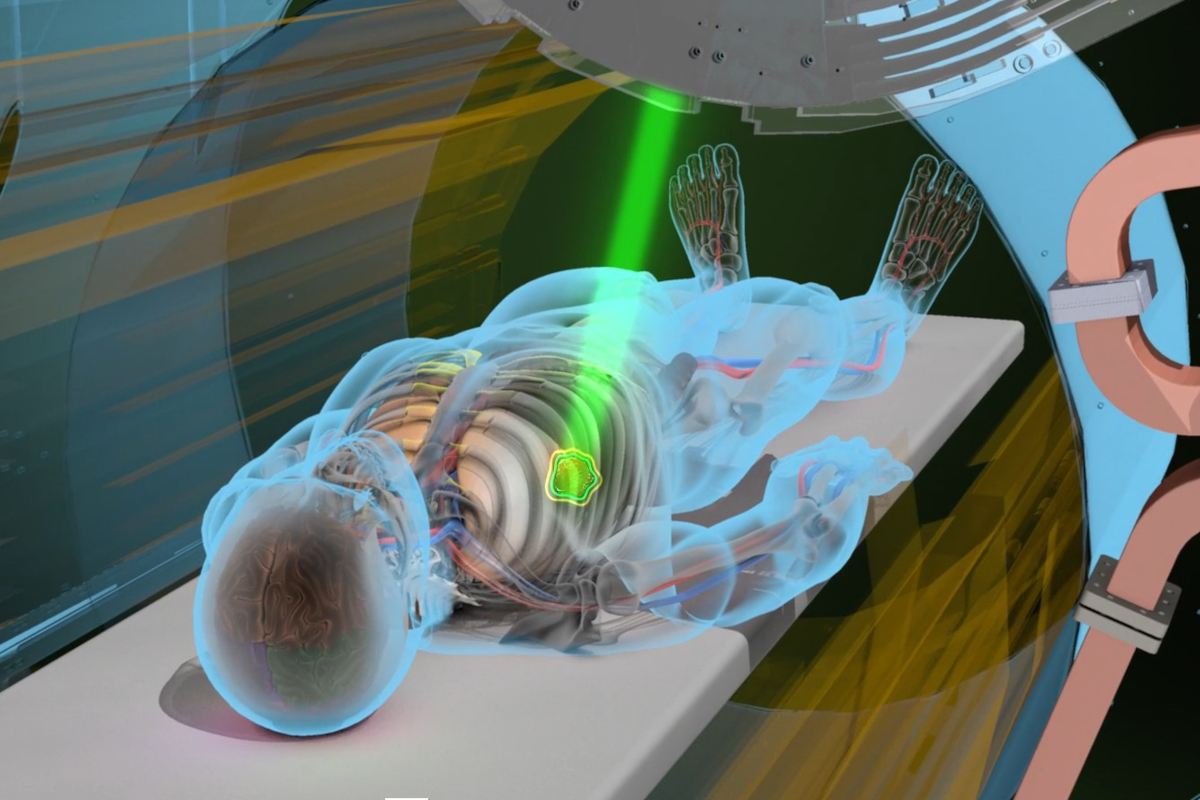
Today, radiation therapy uses beams of ionizing radiation to damage the DNA of cancer cells and stop tumours from growing. The patient lies on a couch while a gantry, which carries a linear accelerator (LINAC), rotates around them and delivers X-ray beams (or proton beams, when greater precision is needed) from several directions. A treatment plan must balance:
the dose delivered to the tumour, which must be high enough to control it; and
the dose delivered to healthy tissue, especially to sensitive organs at risk, which must be kept below safe limits.
Beam angle optimization (BAO) is the problem of choosing the set of beam directions that best achieves this balance. It is a hard combinatorial problem, and it has motivated many optimization and machine-learning approaches.
In this project you will work with real (anonymized) clinical CT scans and contours of head-and-neck cancer patients from the OpenKBP challenge [1]. You will build a simple physical model of radiation beams, and use search and reinforcement learning to choose beam angles.
Learning Objectives#
Explain how megavoltage X-rays deposit dose in tissue, and how this differs for protons.
Load and visualize 3D medical imaging data with organ and tumour masks.
Build a physics-based model of a radiation beam, including attenuation in tissue.
Formulate beam-angle selection as an optimization problem with a reward based on dose objectives, and solve it with a greedy search and with reinforcement learning (Q-learning).
Critically compare a learning method with simple baselines.
Data Sources#
The data are a subset of 10 patients from the OpenKBP challenge dataset [1], [2], which contains 340 head-and-neck cancer patients treated with intensity-modulated radiation therapy.
Course mirror: https://courses.physics.illinois.edu/phys498mlp/sp2025/data/projects/RadioTherapy/openkbp_patient_data.zip (14 MB)
Each patient folder (pt_1, pt_2, …) contains CSV files describing a 128 × 128 × 128 voxel volume. Each file lists the flattened voxel indices of the non-zero voxels (first column), and for ct and dose also the values (column data).
ct.csv: the CT scan. The values are CT numbers offset so that air ≈ 0 and water/soft tissue ≈ 1000, i.e. approximately Hounsfield units + 1000.dose.csv: the clinical dose distribution (in Gy) that was actually planned for this patient.PTV56.csv,PTV63.csv,PTV70.csv: planning target volumes, masks of the regions to be treated, prescribed 56, 63 and 70 Gy.PTV70is the primary (highest-risk) tumour volume. We use it as the target.Organs at risk (not every patient has all of them):
SpinalCord.csv: irradiating the spinal cord can cause radiation myelopathy.Brainstem.csv: brainstem injury can have devastating neurological effects.LeftParotid.csv,RightParotid.csv: irradiating these salivary glands can cause xerostomia (dry mouth).Mandible.csv: the mandible has a limited blood supply, and osteoradionecrosis can occur years after treatment.Esophagus.csv,Larynx.csvfor some patients.
possible_dose_mask.csv: voxels where dose can be non-zero (inside the body).voxel_dimensions.csv: voxel size in mm (3.906 × 3.906 × 2.5).
In the arrays below, volume[:, :, k] is an axial slice.
Questions#
Answer each question in a markdown cell directly below it (add code cells where needed). For the background questions, aim for one to two well-organized paragraphs, and cite your sources. Your notebook should run from top to bottom without errors.
Question 01: Absorption & Scattering#
A narrow beam of X-rays is attenuated exponentially as it passes through matter (the Beer–Lambert law):
where \(x\) is the depth in the body, \(I(x)\) the beam intensity at depth \(x\), \(I_0\) the intensity at the skin, and \(\mu\) the linear attenuation coefficient. \(\mu\) depends on the photon energy and on the tissue traversed (bone, soft tissue, lung, …).
Which physical processes cause this loss of intensity? Name at least three.
Which one dominates for a typical 6 MV radiotherapy beam? The photons in such a beam have a spectrum of energies up to 6 MeV, with a mean of about 2 MeV. Use the NIST attenuation data for water [5] to estimate \(\mu\) for 2 MeV photons, and the fraction of the beam remaining after 10 cm of water.
It is easy to conclude from the formula that the highest dose is delivered at the skin. Why is this not true for megavoltage photon beams? (Hint: look up the “build-up region” of a depth-dose curve.)
Question 02: Dosimetry#
We quantify the effect of radiation on tissue, healthy or cancerous, by the absorbed dose: the energy deposited per unit mass, measured in gray (1 Gy = 1 J/kg):
What are the consequences of delivering too little or too much dose? Does the type of tissue matter?
Clinical plans respect dose limits for each organ at risk. Find typical limits for the spinal cord, brainstem and parotid glands, e.g. from the QUANTEC reviews [3], [4].
Putting it all together, which factors determine the ideal beam angles? Why is choosing them a hard optimization problem? How many ways are there to choose 5 beams out of 36 possible angles?
Question 03: Proton Therapy#
If we used protons instead of X-rays, how would the dose deposited along the beam differ (hint: Bragg peak), and how would that change our beam-angle considerations?
Question 04: Preparing Tensors#
Download and unzip the data with the cell below, then load the patients. The provided functions convert each CSV file into a dense 3D array.
Complete the loop so that, for each patient, the CT, the target (
PTV70), and the organs at risk are stacked into a single array with a leading channel dimension. Use a zero mask for any organ that is missing for a patient. What is the final shape? Draw an analogy to an RGB image.Visualize an axial slice through the target for a few patients: the CT in grayscale, with the contours of the target and of the organs at risk overlaid. Next to it, show the clinical dose distribution (
dose.csv) on the same slice. Which features of the clinical dose do you notice?
import os, urllib.request, zipfile
if not os.path.isdir("openkbp_patient_data"):
    urllib.request.urlretrieve("https://courses.physics.illinois.edu/phys498mlp/sp2025/data/projects/RadioTherapy/openkbp_patient_data.zip", "openkbp_patient_data.zip")
    with zipfile.ZipFile("openkbp_patient_data.zip") as z:
        z.extractall("openkbp_patient_data", members=[m for m in z.namelist() if not m.startswith("__MACOSX")])
import numpy as np
import pandas as pd
import matplotlib.pyplot as plt

base_path = "openkbp_patient_data"
SHAPE = (128, 128, 128)
patient_ids = ["pt_1", "pt_2", "pt_9", "pt_40", "pt_68", "pt_70", "pt_90", "pt_91", "pt_99", "pt_187"]
ORGANS = ["SpinalCord", "Brainstem", "LeftParotid", "RightParotid", "Mandible"]

def load_volume(path, values=False):
    """Convert an OpenKBP sparse CSV file into a dense 128x128x128 array (mask, or values if values=True)."""
    df = pd.read_csv(path, index_col=0)
    flat = np.zeros(np.prod(SHAPE), dtype=np.float32)
    flat[df.index.values] = df["data"].values if values else 1.0
    return flat.reshape(SHAPE)

PIXEL_MM = float(np.loadtxt(os.path.join(base_path, patient_ids[0], "voxel_dimensions.csv"))[0])
print("pixel size:", PIXEL_MM, "mm")
patients = {}
for pt_id in patient_ids:
    pt_dir = os.path.join(base_path, pt_id)
    ct   = load_volume(os.path.join(pt_dir, "ct.csv"), values=True)
    dose = load_volume(os.path.join(pt_dir, "dose.csv"), values=True)
    ptv  = load_volume(os.path.join(pt_dir, "PTV70.csv"))
    oars = {}
    for organ in ORGANS:
        path = os.path.join(pt_dir, f"{organ}.csv")
        oars[organ] = load_volume(path) if os.path.exists(path) else np.zeros(SHAPE, np.float32)

    pt_tensor = ...  # YOUR CODE HERE: stack ct, ptv and the organ masks along a new first (channel) axis
    patients[pt_id] = {"tensor": pt_tensor, "dose": dose}

# YOUR CODE HERE: visualization
For the rest of the project we work with one 2D axial slice per patient: the slice in which the target has its largest area. The helper below extracts it.
def get_slice(pt_id):
    """Return the CT, target mask, organ masks (dict) and clinical dose on the axial slice with the largest target area."""
    t = patients[pt_id]["tensor"]
    k = int(np.argmax(t[1].sum(axis=(0, 1))))
    organs = {name: t[2 + i][:, :, k] for i, name in enumerate(ORGANS)}
    return t[0][:, :, k], t[1][:, :, k], organs, patients[pt_id]["dose"][:, :, k]
Modelling radiation beams#
We model each beam on a 2D slice. A beam is aimed at the centre of the target from a direction given by its gantry angle, one of 36 possible angles (one every 10°). It enters the body from the source side, and the dose it deposits decreases with depth.
The function straight_beam below is a first, naive model: a beam of constant intensity and a fixed width (a Gaussian profile across the beam) inside the body, with no attenuation. You will add physics in Question 06. Note how the geometry is computed: each pixel’s position is projected onto the beam axis and onto the perpendicular direction. This automatically handles any angle correctly.
from scipy.ndimage import center_of_mass, map_coordinates

ANGLES = np.arange(0, 360, 10)

def beam_geometry(angle_deg, target):
    """For every pixel: distance along the beam axis (pixels, negative = source side) and perpendicular distance,
    for a beam aimed at the target centroid from direction angle_deg."""
    c = np.array(center_of_mass(target))
    a = np.deg2rad(angle_deg)
    d = np.array([np.sin(a), np.cos(a)])                  # direction of travel (row, col)
    R, C = np.mgrid[0:target.shape[0], 0:target.shape[1]]
    rel = np.stack([R - c[0], C - c[1]], axis=-1)
    along = rel @ d
    perp = rel @ np.array([-d[1], d[0]])
    return c, d, along, perp

def straight_beam(angle_deg, ct, target, sigma_mm=4.0):
    """Naive beam: constant intensity along the beam, Gaussian lateral profile, zero outside the body."""
    _, _, along, perp = beam_geometry(angle_deg, target)
    body = ct > 200
    return np.exp(-0.5 * (perp * PIXEL_MM / sigma_mm) ** 2) * body
Question 05: Choosing beam angles: reward, search, and reinforcement learning#
A treatment plan here consists of N_BEAMS = 5 distinct beam angles. Its dose is the sum of the doses of its beams. To compare plans, we normalize each plan’s dose so that the mean dose in the target equals 1, which represents the prescription dose. Dose limits for organs are then expressed as fractions of the prescription (e.g. 54 Gy / 70 Gy ≈ 0.77).
Reward. Write a function
reward(dose, target, organs, ct)that returns a single score (higher is better) for a plan. It should:penalize underdose in the target, e.g. the mean of \(\max(0,\ 0.95 - D)\) over target pixels;
penalize overdose in each organ at risk above its limit (Question 02), e.g. the mean of \(\max(0,\ D - D_\text{limit})\) over the organ’s pixels, skipping organs absent from the slice;
mildly penalize the mean dose to the rest of the body (healthy tissue).
Choose and justify weights for the terms.
Baselines. For one patient, evaluate (a) many random 5-beam plans and (b) a greedy search: choose the single best beam, then the best second beam given the first, and so on. Report the rewards.
Reinforcement learning. Implement tabular Q-learning with an \(\epsilon\)-greedy policy. A short introduction: the agent keeps a value \(Q(a)\) for each beam angle \(a\). In each episode it builds a plan by choosing 5 distinct angles, picking a random angle with probability \(\epsilon\) (exploration) and otherwise the angle with the highest \(Q\) among those not yet chosen (exploitation). It then evaluates the plan’s reward \(r\) and updates each chosen angle with \(Q(a) \leftarrow Q(a) + \alpha\,[r - Q(a)]\). (Because there is no state that changes between decisions, this is a so-called multi-armed bandit version of Q-learning. See Ref. [6], Chapters 2 and 6, and the reinforcement learning lecture notebook from a previous edition of this course.)
Train it, plot the reward per episode, print the 5 angles with the highest \(Q\), and visualize the resulting plan on the CT slice.
Compare the plans found by random search, greedy search and Q-learning, both by reward and visually. Which works best, and why? What is a weakness of giving every beam in a plan the same reward?
N_BEAMS = 5
DOSE_LIMITS = {        # fraction of the 70 Gy prescription; replace with your values from Question 02
    "SpinalCord": 50 / 70,
    "Brainstem": 54 / 70,
    "LeftParotid": 25 / 70,
    "RightParotid": 25 / 70,
    "Mandible": 70 / 70,
}

def plan_dose(angles, ct, target, beam_fn):
    return sum(beam_fn(a, ct, target) for a in angles)

def show_plan(angles, pt_id, beam_fn, title=""):
    ct, target, organs, _ = get_slice(pt_id)
    dose = plan_dose(angles, ct, target, beam_fn)
    dose = dose / dose[target > 0].mean()
    plt.figure(figsize=(6, 6))
    plt.imshow(ct, cmap="gray")
    plt.imshow(np.ma.masked_where(dose < 0.05, dose), cmap="hot", alpha=0.5)
    plt.contour(target, colors="lime", linewidths=1)
    for m in organs.values():
        if m.sum() > 0:
            plt.contour(m, colors="cyan", linewidths=1)
    plt.title(f"{title} beams: {sorted(int(a) for a in angles)}\ntarget: green, organs at risk: cyan")
    plt.axis("off"); plt.show()
def reward(dose, target, organs, ct):
    # YOUR CODE HERE
    raise NotImplementedError

# YOUR CODE HERE: random plans, greedy search, Q-learning, comparison
Question 06: A physics-informed beam#
Now make the beam more realistic, using what you learned in Question 01. Implement physical_beam(angle_deg, ct, target), in which the intensity decreases with the radiological depth, i.e. the tissue the beam has traversed from where it enters the body:
Use \(\mu_\text{water} \approx 0.0049\) mm\(^{-1}\), appropriate for a 6 MV beam (Question 01). Take the relative density \(\rho_\text{rel}\) ≈ CT value / 1000, clipped at 0. Remember that one pixel is
PIXEL_MMmm.Hint: use
beam_geometryto get the beam axis. Sample \(\rho_\text{rel}\) along the central axis of the beam (e.g. withscipy.ndimage.map_coordinates), and accumulate it withnp.cumsum. Then assign each pixel the attenuation at its distance along the axis (along), e.g. withnp.interp. Keep the Gaussian lateral profile and the body mask fromstraight_beam.
Then:
Plot the dose of a single physical beam, and its profile along the beam axis. Compare it with
straight_beam, and with the depth-dose behaviour you discussed in Question 01. Which physics is still missing from this model?Repeat the greedy search and the Q-learning of Question 05 with
physical_beam. Do the chosen angles change? Why does the direction a beam enters from now matter, whereas forstraight_beamthe angles \(\theta\) and \(\theta + 180°\) give the same dose?In the clinic, each beam is shaped by collimators to cover the whole target. Experiment with the beam width (
sigma_mm): how do the target coverage and the organ doses change, and which width is sensible for this patient?Apply your best method to several patients and show the plans. Compare them qualitatively with the clinical dose distributions (Question 04). Real clinical plans use many more beams with modulated intensities, so do not expect them to match.
MU_WATER = 0.0049   # 1/mm, 6 MV beam in water

def physical_beam(angle_deg, ct, target, sigma_mm=4.0):
    # YOUR CODE HERE
    raise NotImplementedError
Question 07: Deep reinforcement learning (optional)#
The bandit version of Q-learning ignores the fact that the value of a beam depends on the beams already chosen. A deep Q-network (DQN) can learn this: let the state be the current partial plan, e.g. the accumulated dose image together with the CT and masks, or a binary vector of the angles chosen so far. Let the action be the next angle, and the reward the improvement in reward when that beam is added. Train a DQN with the usual Bellman (temporal-difference) loss.
Where does the physics belong? One might be tempted to add a “physics loss” (e.g. target underdose plus organ overdose) directly to the Bellman loss. Explain why this does not work: the dose of a plan depends on discrete chosen angles, so such a term has no gradient with respect to the network parameters. Instead, physics enters through the reward (as in Question 05), and through the physical beam model.
Train your DQN on several patients, and test it on a patient it has not seen. Does it generalize? How does it compare with the greedy search?
Further ideas (optional)#
Dose prediction (the original OpenKBP task [1]): train a CNN (e.g. a small U-Net) to predict the clinical dose slice from the CT and the masks. With only 10 patients, use 2D slices and data augmentation, and evaluate on held-out patients. The full OpenKBP dataset (340 patients) is available from Ref. [2].
Make the beam model 3D, or include the build-up region and scattered dose.
Use the dose-volume histograms (DVHs) of the target and organs, the standard clinical tool, to compare plans.
References#
[1] A. Babier, B. Zhang, R. Mahmood, K. L. Moore, T. G. Purdie, A. L. McNiven, T. C. Y. Chan, “OpenKBP: The open-access knowledge-based planning grand challenge and dataset,” Med. Phys. 48, 5549 (2021). doi:10.1002/mp.14845
[2] OpenKBP code and data repository. ababier/open-kbp
[3] S. M. Bentzen et al., “Quantitative Analyses of Normal Tissue Effects in the Clinic (QUANTEC): An Introduction to the Scientific Issues,” Int. J. Radiat. Oncol. Biol. Phys. 76, S3 (2010). doi:10.1016/j.ijrobp.2009.09.040
[4] L. B. Marks et al., “Use of Normal Tissue Complication Probability Models in the Clinic,” Int. J. Radiat. Oncol. Biol. Phys. 76, S10 (2010). doi:10.1016/j.ijrobp.2009.07.1754
[5] J. H. Hubbell, S. M. Seltzer, “X-Ray Mass Attenuation Coefficients,” NIST Standard Reference Database 126: water. https://physics.nist.gov/PhysRefData/XrayMassCoef/ComTab/water.html
[6] R. S. Sutton, A. G. Barto, Reinforcement Learning: An Introduction, 2nd ed. (MIT Press, 2018). http://incompleteideas.net/book/the-book-2nd.html
Acknowledgements#
Initial version: Aarya Mehta with some guidance from Mark Neubauer
Revised: 2026
© Copyright 2026