
Anisotropy in the Quark-Gluon Plasma#
Overview#
In Project 01 you characterized the shapes of TRENTO initial states [2], built a Monte Carlo model of jet energy loss in the QGP [3], and made a first prediction of the jet \(v_2\) measured by ATLAS [4]. In this project you will:
fit the energy-loss model to the ATLAS data with an optimization method, and quantify the uncertainty of the fitted parameters;
study how each event’s jet \(v_2\) is related to its initial eccentricity \(\varepsilon_2\); and
train a convolutional neural network (CNN) to act as a fast surrogate for the jet simulation, predicting an event’s jet \(v_2\) directly from its initial-state image.
Reuse your functions from Project 01 (vn, the eccentricity calculation, the centrality selection, the power-law jet spectrum, and eloss).
Data Sources#
TRENTO initial states [2]: https://courses.physics.illinois.edu/phys498mlp/sp2024/data/projects/AnisotropyQGP/events.hdf (208 MB). This is an HDF5 file in the standard TRENTO output format (see the TRENTO documentation). It contains 10,000 minimum-bias Pb+Pb events,
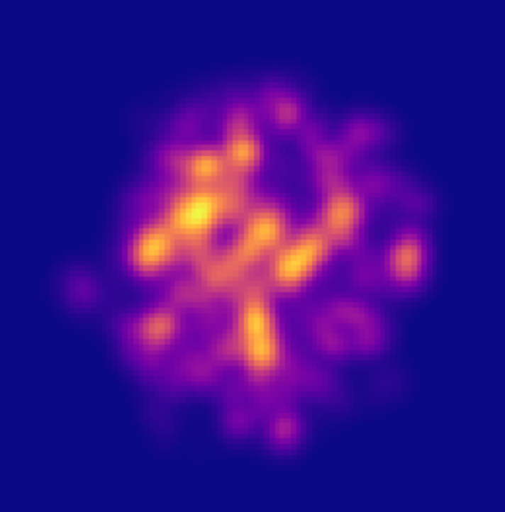
event_0…event_9999. Each event is a 100 × 100 grid covering −10 fm < x, y < 10 fm in 0.2 fm cells, and stores the event properties as attributes: impact parameterb(fm), number of participantsnpart, integrated reduced thicknessmult, and eccentricitiese2–e5.Jet energies: https://courses.physics.illinois.edu/phys498mlp/sp2024/data/projects/AnisotropyQGP/jet_energy.txt (35 MB). One jet energy (GeV) per line, 4.68 million values. Look at it carefully in Project 01, Question 07.
ATLAS jet \(v_2\) measurement [4]: digitized values for 5–10% centrality are given in the code below. The exact published values are available from HEPData.
%matplotlib inline

import os
import urllib.request

import numpy as np
import matplotlib.pyplot as plt
import h5py

BASE_URL = "https://courses.physics.illinois.edu/phys498mlp/sp2024/data/projects/AnisotropyQGP/"

def fetch(filename):
    """Download a file from the course mirror once; later calls reuse the local copy."""
    if not os.path.exists(filename):
        urllib.request.urlretrieve(BASE_URL + filename, filename)
    return filename

events = h5py.File(fetch("events.hdf"), "r")
jet_energy = np.loadtxt(fetch("jet_energy.txt"))

GRID_STEP = 0.2                                   # fm per cell
grid_x = (np.arange(100) - 49.5) * GRID_STEP      # cell-centre coordinates in fm, from -9.9 to +9.9

print(len(events), "TRENTO events;", len(jet_energy), "jet energies")
print(dict(events["event_0"].attrs))


# ATLAS jet v2 for 5-10% centrality Pb+Pb collisions, Fig. 7 of Ref. [4], digitized with https://plotdigitizer.com/app.
# Exact values (with separate statistical and systematic uncertainties) are available on HEPData (record ins1967021).
pt_bin_edges = np.array([71, 79, 89, 100, 126, 158, 200, 251, 316, 398])   # GeV; 9 bins
v2_values = np.array([0.0248856, 0.0221773, 0.0195450, 0.0180492, 0.0178510,
                      0.0086814, 0.0120297, 0.0036979, 0.0138812])
v2_errors = np.array([0.0050671, 0.0049263, 0.0042100, 0.0038375, 0.0038205,
                      0.0041046, 0.0048910, 0.0053504, 0.0092933])
Questions#
General instructions
Answer each question in a markdown cell directly below it (add code cells where needed). Your notebook should run from top to bottom without errors.
Fix your random seeds, so that your results are reproducible.
For the neural networks, use PyTorch, as in the Convolutional and Recurrent Neural Networks, Deep Learning and GPU 101 lectures. Keep separate training, validation and test sets. Plot training and validation loss versus epoch, and report the number of trainable parameters, the training time and the hardware used.
Question 01#
Fitting the energy-loss model. Using an optimization method discussed in class, find the parameters of the energy-loss model that best describe the ATLAS 5–10% data (Fig. 7 of Ref. [4], values in the cell above). Minimize a \(\chi^2\) that includes both the experimental uncertainties and the statistical uncertainty of your simulation.
Things to think about:
Your objective function is noisy, because it is computed from a Monte Carlo simulation. Gradient-based optimizers can be confused by this. Use a fixed random seed for every evaluation (“common random numbers”), so that the objective is a smooth function of the parameters. Consider a gradient-free method (e.g. Nelder–Mead), a grid scan, or Bayesian optimization.
Not all parameters can be determined from \(v_2\) alone. For example, the TRENTO density has an arbitrary overall normalization. How is \(\kappa\) related to it? Start by fitting \(\kappa\) with the pQCD exponents (\(\alpha = 0\), \(\beta = 3/4\), \(\gamma = 1\)) fixed. Then free one exponent at a time, and explain which parameters the data constrain.
Which \(p_T\) bins to use: remember what you learned about the jet sample in Project 01, Question 07.
What are your best-fit values? Plot your model’s predicted \(v_2\) together with the ATLAS data, and compare the inclusive 71–398 GeV value with Fig. 8 of Ref. [4].
Question 02#
Parameter uncertainties. Estimate the uncertainty of your fitted parameter(s). Use either the curvature of \(\chi^2\) near its minimum (\(\Delta\chi^2 = 1\)), or a bootstrap, in which you refit pseudo-datasets generated by fluctuating the ATLAS points within their uncertainties. Optional: sample the posterior distribution of the parameters with MCMC (e.g. emcee), as in the Bayesian Statistics and Markov Chain Monte Carlo lecture, and show the corner plot.
Question 03#
Eccentricity and jet \(v_2\), event by event. With your best-fit parameters, compute the jet \(v_2\) (inclusive 71–398 GeV, relative to each event’s own \(\Phi_2\)) for each TRENTO event in the 0–50% centrality range. Use enough jets per event (several thousand) that the statistical uncertainty on each event’s \(v_2\) is small compared with the spread between events.
Plot \(v_2\) versus \(\varepsilon_2\), and compute their correlation coefficient. Colour the points by centrality.
Is the relation approximately linear (\(v_2 \approx k\,\varepsilon_2\))? How much of the scatter is due to the finite number of jets per event, and how much is physical? (Hint: compare the scatter with \(1/\sqrt{2N_{\rm jets}}\).)
Is \(\varepsilon_2\) alone a good predictor of jet \(v_2\), or does the event size (
mult) also matter?
Question 04#
A CNN surrogate for the jet simulation. The jet simulation is slow, because each event needs thousands of jets. Train a convolutional neural network that takes a TRENTO image (100 × 100 grid) as input and predicts that event’s jet \(v_2\). Use the per-event values from Question 03 as training targets; you may need to simulate more events to have enough training data.
Describe your network and its input preprocessing. Should the input be normalized per event, or would that remove useful information? Can you exploit symmetries, for example by rotating or reflecting images (and correspondingly \(\Phi_2\)) for data augmentation, since \(v_2\) is defined relative to the event’s own \(\Phi_2\)?
Your training targets are noisy, because each one comes from a finite number of jets. Explain why a network trained with a mean-squared-error loss still learns the expected \(v_2\). Compare the network’s test-set error with the statistical noise of the targets.
Plot predicted versus simulated \(v_2\) on the test set. Repeat the \(v_2\)-versus-\(\varepsilon_2\) plot of Question 03 using the CNN predictions. Is it similar?
How much faster is the CNN than the simulation? How could such a surrogate be used, for example in the fit of Question 01?
Optional extension: generating initial states. Train a conditional generative model that produces new 100 × 100 TRENTO-like initial-state grids from a requested set of eccentricities \(\varepsilon_2\)–\(\varepsilon_5\). You may also want to condition on mult, since the eccentricities alone do not fix the size of the event. Generative models such as variational autoencoders and GANs are introduced in the Unsupervised Learning lecture.
A successful model should produce events whose eccentricities, computed with your function from Project 01, match the requested values, and which look like real TRENTO events. Compute the jet \(v_2\) of some generated events, either with the simulation or with your CNN surrogate, and compare the \(v_2\)-versus-\(\varepsilon_2\) correlation with that of Question 03.
References#
[1] S. A. Voloshin, A. M. Poskanzer, R. Snellings, “Collective phenomena in non-central nuclear collisions,” in Relativistic Heavy Ion Physics, Landolt-Börnstein I/23, 293 (Springer, 2010). doi:10.1007/978-3-642-01539-7_10, arXiv:0809.2949
[2] J. S. Moreland, J. E. Bernhard, S. A. Bass, “Alternative ansatz to wounded nucleon and binary collision scaling in high-energy nuclear collisions,” Phys. Rev. C 92, 011901 (2015). doi:10.1103/PhysRevC.92.011901, arXiv:1412.4708. Code documentation: http://qcd.phy.duke.edu/trento/
[3] B. Betz, F. Senzel, C. Greiner, M. Gyulassy, “The impact of the medium and the jet-medium coupling on jet measurements at RHIC and LHC,” arXiv preprint (2015). arXiv:1512.07443
[4] ATLAS Collaboration, “Measurements of azimuthal anisotropies of jet production in Pb+Pb collisions at √sNN = 5.02 TeV with the ATLAS detector,” Phys. Rev. C 105, 064903 (2022). doi:10.1103/PhysRevC.105.064903, arXiv:2111.06606. Numerical data: HEPData
[5] W. Busza, K. Rajagopal, W. van der Schee, “Heavy Ion Collisions: The Big Picture, and the Big Questions,” Ann. Rev. Nucl. Part. Sci. 68, 339 (2018). doi:10.1146/annurev-nucl-101917-020852, arXiv:1802.04801
Acknowledgements#
Initial version: Abraham Holterman with some guidance from Mark Neubauer
Revised: 2026
© Copyright 2026