Artificial Intelligence and Machine Learning#
Overview#
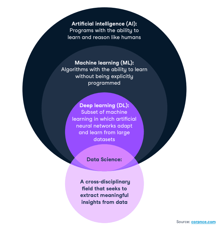
There is no consensus on the precise definitions of data science, machine learning, deep learning and artificial intelligence. For our purposes, we consider the following definitions:
Data Science (DS): a cross-disciplinary field that employs scientific approaches, processes, algorithms and systems used to extract meaning and insights from data.
Artificial Intelligence (AI): a field of research aiming to develop artificial systems with human-level learning and reasoning abilities, possessing the qualities of intentionality, intelligence and adaptability.
Machine Learning (ML): a subset of the field of AI which involves algorithms with the ability to learn without being explicitly programmed. These algorithms learn from data to improve their accuracy, adaptability and utility.
A little ML history: Arthur Samuel is an American computer scientist who is credited for coining the term, “machine learning” with his research in computer systems at UIUC (he initiated the ILLIAC project) then at IBM where he developed the first checkers program on IBM’s first commercial computer in 1959. Robert Nealey, a self-proclaimed checkers master, played the game on an IBM 7094 computer in 1962, and he lost to the computer. Compared to what can be done today, this feat seems trivial, but it’s considered a major milestone in the field of artificial intelligence.
Artificial neural networks (ANNs): comprised of node layers, containing an input layer, one or more hidden layers, and an output layer. Each node, or artificial neuron, connects to another and has an associated weight and threshold. If the output of any individual node is above the specified threshold value, that node is activated, sending data to the next layer of the network. Otherwise, no data is passed along to the next layer of the network by that node.
Deep Learning (DL): a subset of ML in which artificial neural networks adapt and learn from large datasets. The “deep” in deep learning is just referring to the number of layers in a neural network. A neural network that consists of more than three layers—which would be inclusive of the input and the output—can be considered a deep learning algorithm or a deep neural network. A neural network that only has three layers is just a basic neural network. You can think of deep learning as “scalable machine learning” that eliminates some of the human intervention required (through flexible frameworks) and enables the use of larger data sets to continually improve the model performance.
The figure below summarizes these definitions and relationships:
Types of Learning#
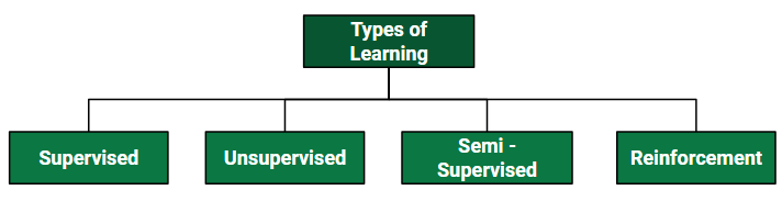
Supervised Learning#
Supervised learning, also known as supervised machine learning, is where machines are taught by example. It is defined by its use of labeled datasets to train algorithms to classify new data or predict outcomes accurately. As input data is fed into the model, the model adjusts its weights until it has been fitted appropriately. This occurs as part of the cross validation process to ensure that the model avoids overfitting or underfitting. Supervised learning helps organizations solve a variety of real-world problems at scale, such as classifying spam in a separate folder from your inbox. Some methods used in supervised learning include neural networks, naïve bayes, linear regression, logistic regression, random forest, and support vector machine (SVM).
There are two main categories of supervised learning that are mentioned below:
Classification: Classification is a process of categorizing data or objects into predefined categories based on their features or attributes and determining to what category new observations belong.
Regression: Regression is a process to estimate the relationships among variables when the output variable is a real or continuous value.
Advantages of Supervised Machine Learning:
Supervised Learning models can have high accuracy as they are trained on labelled data.
The process of decision-making in supervised learning models is often interpretable.
It can often be used in pre-trained models which saves time and resources when developing new models from scratch.
Disadvantages of Supervised Machine Learning:
It has limitations in knowing patterns and may struggle with unseen or unexpected patterns that are not present in the training data.
It can be time-consuming and costly as it relies on labeled data only.
It may lead to poor generalizations based on new data.
Unsupervised Learning#
Unsupervised learning is a machine learning technique in which an algorithm discovers patterns and relationships using unlabeled data. Unlike supervised learning, unsupervised learning doesn’t involve providing the algorithm with labeled target outputs. The primary goal of Unsupervised learning is often to discover hidden patterns, similarities, or clusters within the data, which can then be used for various purposes, such as data exploration, visualization, dimensionality reduction, and more.
There are two main categories of unsupervised learning that we have already studied extensively:
Clustering: Clustering is the task of dividing the population or data points into a number of groups such that data points in the same groups are more similar to other data points in the same group and dissimilar to the data points in other groups. It is basically a collection of objects on the basis of similarity and dissimilarity between them.
Dimensionality Reduction: Dimensionality reduction is a technique used to reduce the number of features in a dataset while retaining as much of the important information as possible. In other words, it is a process of transforming high-dimensional data into a lower-dimensional space that still preserves the essence of the original data. This can be done for a variety of reasons, such as to reduce the complexity of a model, to improve the performance of a learning algorithm, or to make it easier to visualize the data.
Advantages of Unsupervised Machine Learning:
It helps to discover hidden patterns and various relationships between the data.
Used for tasks such as anomaly detection and data exploration. Techniques such as autoencoders and dimensionality reduction that can be used to extract meaningful features from raw data.
It does not require labeled data and reduces the effort of data labeling.
Disadvantages of Unsupervised Machine Learning:
Without using labels, it may be difficult to predict the quality of the model’s output.
Cluster Interpretability may not be clear and may not have meaningful interpretations.
Semi-Supervised Learning#
Semi-supervised learning is a type of machine learning that falls in between supervised and unsupervised learning. It is a method that uses a small amount of labeled data and a large amount of unlabeled data to train a model. The goal of semi-supervised learning is to learn a function that can accurately predict the output variable based on the input variables, similar to supervised learning. However, unlike supervised learning, the algorithm is trained on a dataset that contains both labeled and unlabeled data. Semi-supervised learning is particularly useful when there is a large amount of unlabeled data available, but it’s too expensive or difficult to label all of it.
Advantages of Semi-supervised Machine Learning:
It leads to better generalization as compared to supervised learning, as it takes both labeled and unlabeled data.
Can be applied to a wide range of data.
Disdvantages of Semi-supervised Machine Learning:
Semi-supervised methods can be more complex to implement compared to other approaches.
It still requires some labeled data that might not always be available or easy to obtain.
The unlabeled data can impact the model performance accordingly.
Reinforcement Learning#
Reinforcement learning is a learning method that interacts with an environment by producing actions and discovering errors. It is the science of decision making - learning the optimal behavior in an environment to obtain maximum reward. Trial, error, and delay are the most relevant characteristics of reinforcement learning. These methods allows machines to become autonomous, self-learners that automatically determine the ideal behaviour within specific context in order to maximize performance. This type of learning is crucial for applications that involve decision-making in unpredictable environments.
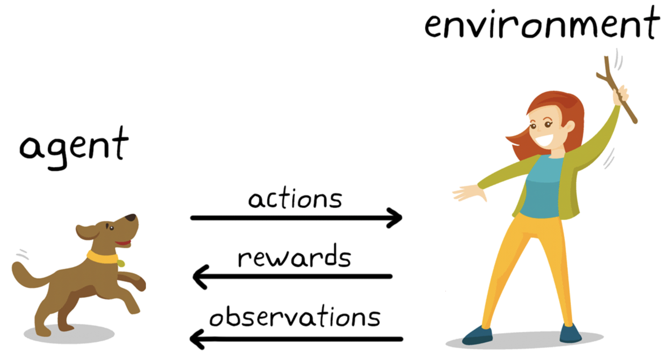
EXAMPLE: Dog training
The goal of learning in this case is to train the dog (agent) to complete a task within an envirnoment, which includes the surroundings of the dog as well as the trainer.
First, the trainer issues a command or cue, which the dog observes (observation)
The dog then responds by taking an action
If the action is close to the desired behavior, the trainer will likely provide a reward, such as a food treat or a toy; otherwise, no reward will be provided.
At the beginning of training, the dog will likely take more random actions like rolling over when the command given is “sit,” as it is trying to associate specific observations with actions and rewards. This association, or mapping, between observations and actions is called policy.
From the dog’s perspective, the ideal case would be one in which it would respond correctly to every cue, so that it gets as many treats as possible. So, the whole meaning of reinforcement learning training is to “tune” the dog’s policy so that it learns the desired behaviors that will maximize some reward.
After training is complete, the dog should be able to observe the owner and take the appropriate action, for example, sitting when commanded to “sit” by using the internal policy it has developed. By this point, treats are welcome but, theoretically, shouldn’t be necessary.
Advantages of Reinforcement Machine Learning:
It has autonomous decision-making that is well-suited for tasks and that can learn to make a sequence of decisions without human guidance, like robotics and game-playing. For promising science and engineering applications, it can be used for beam controls in particle acclerators, steering of high-temperature plasma in fusion systems, just to name a few.
This technique is preferred to achieve long-term results that are very difficult to achieve.
It is used to solve a complex problems that cannot be solved by conventional techniques.
Disadvantages of Reinforcement Machine Learning:
Training Reinforcement Learning agents can be computationally expensive and time-consuming.
Reinforcement learning is not preferable to solving simple problems.
It needs a lot of data and a lot of computation, which makes it impractical and costly.
Acknowledgments#
Initial version: Mark Neubauer
© Copyright 2025