Homework 02: Visualization and Expectation-Maximization#
%matplotlib inline
import matplotlib.pyplot as plt
import seaborn as sns; sns.set_theme()
import numpy as np
import pandas as pd
import os.path
import subprocess
Helpers for Getting, Loading and Locating Data
def wget_data(url: str):
    local_path = './tmp_data'
    p = subprocess.Popen(["wget", "-nc", "-P", local_path, url], stderr=subprocess.PIPE, encoding='UTF-8')
    rc = None
    while rc is None:
      line = p.stderr.readline().strip('\n')
      if len(line) > 0:
        print(line)
      rc = p.poll()

def locate_data(name, check_exists=True):
    local_path='./tmp_data'
    path = os.path.join(local_path, name)
    if check_exists and not os.path.exists(path):
        raise RuxntimeError('No such data file: {}'.format(path))
    return path
wget_data('https://raw.githubusercontent.com/illinois-ipaml/MachineLearningForPhysics/main/data/pong_data.hf5')
wget_data('https://raw.githubusercontent.com/illinois-ipaml/MachineLearningForPhysics/main/data/pong_targets.hf5')
pong_data    = pd.read_hdf(locate_data('pong_data.hf5'))
pong_targets = pd.read_hdf(locate_data('pong_targets.hf5'))
Problem 1#
We often coerce data for machine learning into a 2D array of samples x features, but this sometimes obscures the natural structure of the data. In these cases, it is helpful to use special-purpose visualizations that know about this natural structure.
Samples of pong_data encode 2D trajectories of a ping-pong ball. Implement the function below to transform one sample into a 2D array of trajectory coordinates suitable for plotting:
def sample_to_trajectory(sample):
    """Reshape a pong data sample of length N into an (x,y) array of shape (2, N/2).

    Parameters
    ----------
    sample : array
        Numpy array of length N.

    Returns
    -------
    array
        Array of length (2, N/2) where the first index is 0, 1 for x, y coordinates.
    """
    assert len(sample) % 2 == 0, 'len(sample) is not divisible by two.'
    # YOUR CODE HERE
    raise NotImplementedError()
# A correct solution should pass these tests.
sample = np.arange(10)
xy = sample_to_trajectory(sample)
assert xy.shape == (2, 5)
assert np.array_equal(xy[0], [0, 1, 2, 3, 4])
assert np.array_equal(xy[1], [5, 6, 7, 8, 9])
Use the function below to plot some samples as trajectories, color coded by their target “grp” value:
def plot_trajectories(nrows=50):
    for row in range(nrows):
        x, y = sample_to_trajectory(pong_data.iloc[row].values)
        grp = int(pong_targets['grp'][row])
        color = 'krb'[grp]
        plt.plot(x, y, ls='-', c=color)
plot_trajectories()
It should be obvious from this plot why the y0 column is all zeros.
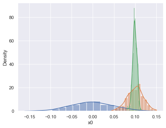
Implement the function below using sns.distplot to show the distribution of x0 values for each value (0, 1, 2) of the target grp. Your plot should resemble this one:
def compare_groups():
    """Plot 1D distributions of the x0 feature for each group (grp=0,1,2).
    """
    # YOUR CODE HERE
    raise NotImplementedError()

compare_groups()
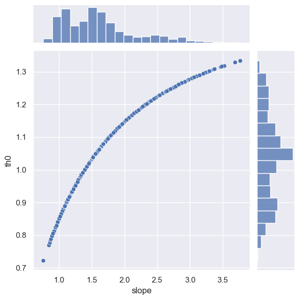
To get some insight into the th0 target, implement the function below to add a slope column to pong_data that calculates the initial trajectory slope, then make a scatter plot of slope versus th0 using sns.jointplot. Your plot should resemble this one:
def compare_slope_th0():
    """Display scatter plot of calculated initial slope vs target th0.
    """
    # YOUR CODE HERE
    raise NotImplementedError()

compare_slope_th0()
Problem 2#
The normal (aka Gaussian) distribution is one of the fundamental probability densities that we will encounter often.
Implement the function below using np.random.multivariate_normal to generate random samples from an arbitrary multidimensional normal distribution, for a specified random seed:
def generate_normal(mu, C, n, seed=123):
    """Generate random samples from a normal distribution.

    Parameters
    ----------
    mu : array
        1D array of mean values of length N.
    C : array
        2D array of covariances of shape (N, N). Must be a positive-definite matrix.
    n : int
        Number of random samples to generate.
    seed : int
        Random number seed to use.

    Returns
    -------
    array
        2D array of shape (n, N) where each row is a random N-dimensional sample.
    """
    assert len(mu.shape) == 1, 'mu must be 1D.'
    assert C.shape == (len(mu), len(mu)), 'C must be N x N.'
    assert np.all(np.linalg.eigvals(C) > 0), 'C must be positive definite.'
    # YOUR CODE HERE
    raise NotImplementedError()
# A correct solution should pass these tests.
mu = np.array([-1., 0., +1.])
C = np.identity(3)
C[0, 1] = C[1, 0] = -0.9
Xa = generate_normal(mu, C, n=500, seed=1)
Xb = generate_normal(mu, C, n=500, seed=1)
Xc = generate_normal(mu, C, n=500, seed=2)
assert np.array_equal(Xa, Xb)
assert not np.array_equal(Xb, Xc)
X = generate_normal(mu, C, n=2000, seed=3)
assert np.allclose(np.mean(X, axis=0), mu, rtol=0.001, atol=0.1)
assert np.allclose(np.cov(X, rowvar=False), C, rtol=0.001, atol=0.1)
Visualize a generated 3D dataset using:
def visualize_3d():
    mu = np.array([-1., 0., +1.])
    C = np.identity(3)
    C[0, 1] = C[1, 0] = -0.9
    X = generate_normal(mu, C, n=2000, seed=3)
    df = pd.DataFrame(X, columns=('x0', 'x1', 'x2'))
    sns.pairplot(df)
visualize_3d()
Read about correlation and covariance, then implement the function below to create a 2x2 covariance matrix given values of \(\sigma_x\), \(\sigma_y\) and the correlation coefficient \(\rho\):
def create_2d_covariance(sigma_x, sigma_y, rho):
    """Create and return the 2x2 covariance matrix specified by the input args.
    """
    assert (sigma_x > 0) and (sigma_y > 0), 'sigmas must be > 0.'
    # YOUR CODE HERE
    raise NotImplementedError()
# A correct solution should pass these tests.
assert np.array_equal(create_2d_covariance(1., 1.,  0.0), [[1.,  0.], [ 0., 1.]])
assert np.array_equal(create_2d_covariance(2., 1.,  0.0), [[4.,  0.], [ 0., 1.]])
assert np.array_equal(create_2d_covariance(2., 1.,  0.5), [[4.,  1.], [ 1., 1.]])
assert np.array_equal(create_2d_covariance(2., 1., -0.5), [[4., -1.], [-1., 1.]])
Run the following cell that uses your create_2d_covariance and generate_normal functions to compare the 2D normal distributions with \(\rho = 0\) (blue), \(\rho = +0.9\) (red) and \(\rho = -0.9\) (green):
def compare_rhos():
    mu = np.zeros(2)
    sigma_x, sigma_y = 2., 1.
    for rho, cmap in zip((0., +0.9, -0.9), ('Blues', 'Reds', 'Greens')):
        C = create_2d_covariance(sigma_x, sigma_y, rho)
        X = generate_normal(mu, C, 10000)
        sns.kdeplot(x=X[:, 0], y=X[:, 1], cmap=cmap)
    plt.xlim(-4, +4)
    plt.ylim(-2, +2)

compare_rhos()
Problem 3#
The Expectation-Maximization (EM) algorithm is used to implement many machine learning methods, including several we have already studied like K-means and soon to be studied (e.g. factor analysis and weighted PCA.)
The basic idea of EM is to optimize a goal function that depends on two disjoint sets of parameters by alternately updating one set and then the other, using a scheme that is guaranteed to improve the goal function (although generally to a local rather than global optimum). The alternating updates are called the E-step and M-step.
The K-means is one of the simplest uses of EM, so is a good way to get some hands-on experience.
Implement the function below to perform a K-means E-step. Hint: you might find np.linalg.norm and np.argmin useful.
def E_step(X, centers):
    """Perform a K-means E-step.

    Assign each sample to the cluster with the nearest center, using the
    Euclidean norm to measure distance between a sample and a cluster center.

    Parameters
    ----------
    X : array with shape (N, D)
        Input data consisting of N samples in D dimensions.
    centers : array with shape (n, D)
        Centers of the the n clusters in D dimensions.

    Returns
    -------
    integer array with shape (N,)
        Cluster index of each sample, in the range 0 to n-1.
    """
    N, D = X.shape
    n = len(centers)
    assert centers.shape[1] == D
    indices = np.empty(N, int)
    # YOUR CODE HERE
    raise NotImplementedError()

    return indices
# A correct solution should pass these tests.
gen = np.random.RandomState(seed=123)
X = gen.normal(size=(100, 2))
centers = np.array([[0., 0.], [0., 10.]])
X[50:] += centers[1]
indices = E_step(X, centers)
assert np.all(indices[:50] == 0)
assert np.all(indices[50:] == 1)

gen = np.random.RandomState(seed=123)
X = gen.normal(size=(20, 2))
centers = gen.uniform(size=(5, 2))
indices = E_step(X, centers)
assert np.array_equal(indices, [4, 1, 4, 4, 1, 0, 1, 0, 2, 1, 2, 4, 0, 1, 0, 1, 0, 1, 4, 4])
Next, implement the function below to perform a K-means M-step:
def M_step(X, indices, n):
    """Perform a K-means M-step.

    Calculate the center of each cluster as the geometric mean of its assigned samples.

    The centers of any clusters without any assigned samples should be set to the origin.

    Parameters
    ----------
    X : array with shape (N, D)
        Input data consisting of N samples in D dimensions.
    indices : integer array with shape (N,)
        Cluster index of each sample, in the range 0 to n-1.
    n : int
        Number of clusters.  Must be <= N.

    Returns
    -------
    array with shape (n, D)
        Centers of the the n clusters in D dimensions.
    """
    N, D = X.shape
    assert indices.shape == (N,)
    assert n <= N
    centers = np.zeros((n, D))
    # YOUR CODE HERE
    raise NotImplementedError()

    return centers
# A correct solution should pass these tests.
gen = np.random.RandomState(seed=123)
X = np.ones((20, 2))
indices = np.zeros(20, int)
centers = M_step(X, indices, 1)
assert np.all(centers == 1.)

n = 5
indices = gen.randint(n, size=len(X))
centers = M_step(X, indices, n)
assert np.all(centers == 1.)

X = gen.uniform(size=X.shape)
centers = M_step(X, indices, n)
assert np.allclose(
    np.round(centers, 3),
    [[ 0.494,  0.381], [ 0.592,  0.645],
     [ 0.571,  0.371], [ 0.234,  0.634],
     [ 0.250,  0.386]])
You have now implemented the core of the K-means algorithm. Try it out with this simple wrapper, which makes a scatter plot of the first two columns after each iteration. The sklearn wrapper combines the result of several random starting points and has other refinements.
def KMeans_fit(data, n_clusters, nsteps, seed=123):
    X = data.values
    N, D = X.shape
    assert n_clusters <= N
    gen = np.random.RandomState(seed=seed)
    # Pick random samples as the initial centers.
    shuffle = gen.permutation(N)
    centers = X[shuffle[:n_clusters]]
    # Perform an initial E step to assign samples to clusters.
    indices = E_step(X, centers)
    # Loop over iterations.
    for i in range(nsteps):
        centers = M_step(X, indices, n_clusters)
        indices = E_step(X, centers)
    # Plot the result.
    cmap = np.array(sns.color_palette())
    plt.scatter(X[:, 0], X[:, 1], c=cmap[indices % len(cmap)])
    plt.scatter(centers[:, 0], centers[:, 1], marker='+', c='k', s=400, lw=5)
    plt.show()
Try it out on some randomly generated 2D data with 3 separate clusters (using the handy make_blobs):
from sklearn.datasets import make_blobs
gen = np.random.RandomState(seed=123)
X, _ = make_blobs(n_samples=500, n_features=2, centers=[[-3,-3],[0,3],[3,-3]], random_state=gen)
data = pd.DataFrame(X, columns=('x0', 'x1'))
For this simple test, you should find a good solution after two iterations:
KMeans_fit(data, n_clusters=3, nsteps=0);
KMeans_fit(data, n_clusters=3, nsteps=1);
KMeans_fit(data, n_clusters=3, nsteps=2);
Acknowledgments#
Initial version: Mark Neubauer
© Copyright 2025