
Searching for Exotic Particles#
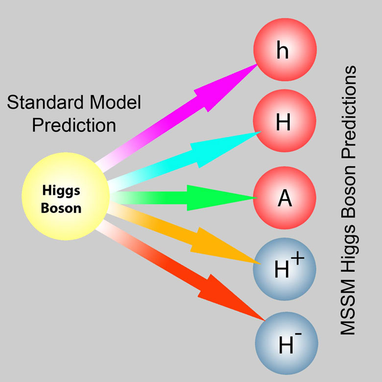
The SM predicts a single Higgs boson. Supersymmetric extensions such as the Minimal Supersymmetric Standard Model (MSSM) predict five: \(h\), \(H\), \(A\) and \(H^\pm\).
Overview#
In Project 01 you explored two benchmark datasets for exotic-particle searches: HIGGS (a heavy neutral Higgs boson decaying via a charged Higgs boson, vs. \(t\bar t\)) and HEPMASS (a new particle \(X\to t\bar t\) of unknown mass, vs. \(t\bar t\)). In this project you will train neural-network classifiers on one of them.
Choose one track:
Track A: HIGGS. Reproduce the main result of Ref. [1]: deep networks trained on low-level features outperform shallow networks, even when the shallow networks are given hand-crafted high-level features.
Track B: HEPMASS. Reproduce the main result of Ref. [2]: a single parameterized network that takes the hypothesized mass \(m_X\) as an input can replace a set of networks trained at fixed masses, and can interpolate to masses it never saw during training.
Data Sources#
The data are the same as in Project 01. See that notebook for the full description, including the header bug in the HEPMASS 1000_* files, which the code below works around.
HIGGS: https://courses.physics.illinois.edu/phys498mlp/sp2025/data/projects/HiggsTauTau/HIGGS.csv.gz (11 million events). There is no header; column 0 is the label, columns 1–21 are low-level features and columns 22–28 are high-level features.
HEPMASS: https://courses.physics.illinois.edu/phys498mlp/sp2025/data/projects/ExoticParticles/hepmass/ (
1000_*,not1000_*andall_*training and test files, with 7 M and 3.5 M events respectively). Column 0 is the label, followed by 27 features (22 low-level, then 5 high-level) and, fornot1000andall, the mass.
The cells below stream only the first N_EVENTS events of each file over the network, so you never need to download the full files. Start small while you develop your code, then increase N_EVENTS for your final results.
import gzip
import urllib.request

import numpy as np
import pandas as pd
import matplotlib.pyplot as plt
from sklearn.model_selection import train_test_split
from sklearn.preprocessing import StandardScaler

BASE_URL = "https://courses.physics.illinois.edu/phys498mlp/sp2025/data/projects/"

def read_events(url, nrows, skip_header=False):
    """Stream the first `nrows` events of a gzipped CSV without downloading all of it."""
    with urllib.request.urlopen(url) as response, gzip.GzipFile(fileobj=response) as f:
        if skip_header:
            f.readline()
        return pd.read_csv(f, header=None, nrows=nrows).to_numpy(dtype=np.float32)
Track A (HIGGS) data
N_EVENTS = 500_000  # increase for your final results

data = read_events(BASE_URL + "HiggsTauTau/HIGGS.csv.gz", N_EVENTS)
X, y = data[:, 1:], data[:, 0]
LOW = list(range(0, 21))    # 21 low-level features
HIGH = list(range(21, 28))  # 7 high-level features

# 60% train / 20% validation / 20% test, stratified by class
X_train, X_tmp, y_train, y_tmp = train_test_split(X, y, test_size=0.4, stratify=y, random_state=42)
X_val, X_test, y_val, y_test = train_test_split(X_tmp, y_tmp, test_size=0.5, stratify=y_tmp, random_state=42)
print({name: a.shape for name, a in [("train", X_train), ("val", X_val), ("test", X_test)]})
Track B (HEPMASS) data
N_EVENTS = 500_000  # per file; increase for your final results
HEP = BASE_URL + "ExoticParticles/hepmass/"

def read_hepmass(name, nrows):
    d = read_events(HEP + name + ".csv.gz", nrows, skip_header=True)  # skip the (buggy) header line
    return d[:, 1:], d[:, 0]   # features (incl. mass column if present), label

X_1000_train, y_1000_train = read_hepmass("1000_train", N_EVENTS)        # 27 features, signal at m_X = 1000 GeV
X_1000_test, y_1000_test = read_hepmass("1000_test", N_EVENTS)
X_not1000_train, y_not1000_train = read_hepmass("not1000_train", N_EVENTS)  # 27 features + mass (500, 750, 1250, 1500 GeV)
X_all_train, y_all_train = read_hepmass("all_train", N_EVENTS)              # 27 features + mass (500 ... 1500 GeV)

print(X_1000_train.shape, X_not1000_train.shape, np.unique(X_not1000_train[:, -1]))
Questions#
General instructions
Use PyTorch, as in the Deep Learning and GPU 101 lectures.
Keep a test set that is never used for training, hyperparameter tuning or early stopping. Use a separate validation set for those.
Fit any input scaling (e.g.
StandardScaler) on the training set only, then apply it to the validation and test sets.Plot training and validation loss versus epoch for every network you train, so you can see whether it has converged or overfit.
For each network, report the number of trainable parameters, the training time, and the hardware used (CPU or GPU model).
The papers trained on tens of millions of events for hundreds of epochs. You are not expected to match their AUC values exactly. Explain any differences you see.
Track A: HIGGS#
Question A1#
Shallow network. Implement and train a shallow neural network (one hidden layer) like those in Ref. [1]. Choose its hyperparameters from the shallow-network options in Supplementary Table 2 of the arXiv version (Supplementary Table 4 of the journal version), or use an even smaller network so that training is manageable on a CPU. Use the complete set of 28 features. The Methods section describes the remaining hyperparameters: tanh hidden units, a logistic output, mini-batches of 100, momentum, and weight decay. You may use a modern optimizer such as Adam instead, but say so.
Show the distribution of the network output for signal and for background test events, overlaid and normalized to unit area, the ROC curve, and the AUC on your test set. Compare with the shallow-network (NN) row of Table 1 of Ref. [1].
Question A2#
Deep network. Train a fully-connected deep neural network on a GPU, with meaningfully more trainable parameters than your shallow network. The paper’s choice was 5 hidden layers of 300 units (see Supplementary Tables 1 and 3 of the arXiv version), but the exact architecture is up to you. Show the same plots and AUC as in Question 01, and overlay the shallow and deep ROC curves on one plot.
Question A3#
Which features matter? Retrain your deep network (and, if time allows, your shallow network) using (a) only the 21 low-level features, (b) only the 7 high-level features, and (c) all 28 features. Summarize the test-set AUCs in a table like Table 1 of Ref. [1].
Does the deep network trained on the low-level features alone recover the information in the high-level features?
How do your conclusions compare with those of the paper?
Track B: HEPMASS#
Question B1#
Fixed-mass network. Train a fully-connected neural network on the 1000 training data (27 features, signal at \(m_X = 1000\) GeV). Set aside part of the training data for validation. Evaluate it on the 1000_test data: show the distribution of the network output for signal and for background test events, overlaid and normalized to unit area, the ROC curve, and the AUC. The architecture used in Ref. [2] was 5 hidden layers of 500 ReLU units with a logistic output. Start with something smaller on a CPU, then scale up on a GPU.
Question B2#
Parameterized network. Train a network on the all training data with the mass as an additional (28th) input. The mass column is in GeV while the other features are normalized, so scale it as well. Remember that background events carry a randomly assigned mass. Evaluate it on 1000_test, appending a mass column set to 1000 GeV for every event.
Then train the same architecture on the not1000 data, which contains no signal events at \(m_X = 1000\) GeV, and evaluate it on 1000_test in the same way. Overlay the ROC curves of all three networks (fixed at 1000 GeV, parameterized on all, parameterized on not1000), as in Fig. 7 of Ref. [2]. Can the parameterized network interpolate to a mass it never saw?
Question B3#
Mass dependence. Your network from Question B2 trained on the all data can be evaluated at any hypothesized mass. Feed the 1000_test events to it with the mass input set in turn to 500, 750, 1000, 1250 and 1500 GeV, and plot the AUC as a function of the input mass. Explain the shape of this curve. Why is the network’s performance best when the input mass matches the true mass of the signal?
Explain in your own words why the parameterized approach is useful in a real search for a particle of unknown mass.
Optional extension (either track): compare your networks with a boosted decision tree (e.g. sklearn.ensemble.HistGradientBoostingClassifier or XGBoost) trained on the same features. BDTs were the standard tool in particle physics at the time.
References#
[1] P. Baldi, P. Sadowski, D. Whiteson, “Searching for exotic particles in high-energy physics with deep learning,” Nature Communications 5, 4308 (2014). doi:10.1038/ncomms5308, arXiv:1402.4735
[2] P. Baldi, K. Cranmer, T. Faucett, P. Sadowski, D. Whiteson, “Parameterized neural networks for high-energy physics,” Eur. Phys. J. C 76, 235 (2016). doi:10.1140/epjc/s10052-016-4099-4, arXiv:1601.07913
[3] D. Whiteson, “HIGGS” [Dataset], UCI Machine Learning Repository (2014). doi:10.24432/C5V312
[4] D. Whiteson, “HEPMASS” [Dataset], UCI Machine Learning Repository (2016). doi:10.24432/C5PP5W
Acknowledgements#
Initial version: Mark Neubauer
Revised: 2026
© Copyright 2026