
Anisotropy in the Quark-Gluon Plasma#
Learning Objectives#
By the end of this project you should be able to:
explain how azimuthal anisotropy (\(v_n\)) arises in heavy-ion collisions, both for low-momentum particles and for high-energy jets;
compute \(v_n\) from a set of particle angles, with and without knowledge of the symmetry plane, and estimate its statistical uncertainty;
read, visualize and characterize simulated initial states of heavy-ion collisions (TRENTO), including centrality selection and eccentricities;
inspect an input dataset critically and discover how it was generated; and
build a simple Monte Carlo model of jet energy loss in the quark-gluon plasma and use it to predict jet \(v_2\).
In Project 02 you will fit this model to ATLAS data and train neural networks on the TRENTO events.
Overview#
The quark-gluon plasma (QGP) is a deconfined state of matter created in heavy-ion collisions at the Large Hadron Collider (LHC) and the Relativistic Heavy Ion Collider (RHIC) [5]. The initial overlap region of the two nuclei is not round, and its shape fluctuates from event to event. The QGP transmits this spatial anisotropy to the final-state particles in two ways:
Low-momentum particles inherit it through the collective, hydrodynamic expansion of the QGP (“flow”).
High-energy jets inherit it because they lose energy while traversing the QGP. Jets that travel through more medium lose more energy, so the jet yield at a given momentum depends on the jet’s direction relative to the shape of the collision region.
Both effects appear as azimuthal anisotropy coefficients \(v_n\) [1]. In this project you will learn how to characterize the shapes of the QGP produced in these collisions, using the TRENTO model of the initial state [2]. You will then use those shapes to build a model of how jets lose energy as they traverse the medium [3], whose predictions you will compare with ATLAS measurements [4].
Data Sources#
TRENTO initial states [2]: https://courses.physics.illinois.edu/phys498mlp/sp2024/data/projects/AnisotropyQGP/events.hdf (208 MB). This is an HDF5 file in the standard TRENTO output format (see the TRENTO documentation). It contains 10,000 minimum-bias Pb+Pb events,
event_0…event_9999. Each event is a 100 × 100 grid covering −10 fm < x, y < 10 fm in 0.2 fm cells, and stores the event properties as attributes: impact parameterb(fm), number of participantsnpart, integrated reduced thicknessmult, and eccentricitiese2–e5.Jet energies: https://courses.physics.illinois.edu/phys498mlp/sp2024/data/projects/AnisotropyQGP/jet_energy.txt (35 MB). One jet energy (GeV) per line, 4.68 million values. Look at it carefully in Project 01, Question 07.
ATLAS jet \(v_2\) measurement [4]: digitized values for 5–10% centrality are given in the code below. The exact published values are available from HEPData.
%matplotlib inline

import os
import urllib.request

import numpy as np
import matplotlib.pyplot as plt
import h5py

BASE_URL = "https://courses.physics.illinois.edu/phys498mlp/sp2024/data/projects/AnisotropyQGP/"

def fetch(filename):
    """Download a file from the course mirror once; later calls reuse the local copy."""
    if not os.path.exists(filename):
        urllib.request.urlretrieve(BASE_URL + filename, filename)
    return filename

events = h5py.File(fetch("events.hdf"), "r")
jet_energy = np.loadtxt(fetch("jet_energy.txt"))

GRID_STEP = 0.2                                   # fm per cell
grid_x = (np.arange(100) - 49.5) * GRID_STEP      # cell-centre coordinates in fm, from -9.9 to +9.9

print(len(events), "TRENTO events;", len(jet_energy), "jet energies")
print(dict(events["event_0"].attrs))
Questions#
Answer each question in a markdown cell directly below it (add code cells where needed). For the background questions, aim for one to two well-organized paragraphs, and cite your sources. Your notebook should run from top to bottom without errors. Fix your random seeds so that your results are reproducible.
Part A: Background#
Question 01#
Read Section 1.2 of Ref. [1].
What are the reaction plane and the participant plane (their Fig. 2), and why do they differ?
Write down the Fourier expansion of the azimuthal particle distribution, their Eq. (1), and explain what \(v_1\), \(v_2\) and \(v_3\) describe.
Their Eq. (2) relates two-particle correlations to \(\langle v_n^2\rangle\). Explain why this is useful in an experiment, where the symmetry plane is not known. What is the “nonflow” term \(\delta_n\)?
Question 02#
What is a jet, and what is meant by jet quenching? Why do jets that traverse more QGP lose more energy, and how does this produce a non-zero jet \(v_2\) in non-central collisions? What is centrality, and how is it determined experimentally? Ref. [4] (Section 1) and Ref. [5] are good starting points.
Part B: Measuring \(v_n\)#
Question 03#
Write a function to evaluate \(v_n\) from an array of particle (or jet) azimuthal angles in two ways:
With a known symmetry plane \(\Psi_n\), using Eq. (1) of Ref. [1]: \(v_n = \langle \cos n(\phi - \Psi_n)\rangle\).
Without knowing \(\Psi_n\), using the two-particle correlation of Eq. (2), assuming the nonflow term \(\delta_n = 0\). (Nonflow comes from correlated particle decays and similar effects, which we will not consider in this project.) With \(Q_n = \sum_j e^{in\phi_j}\) for \(M\) particles, the average over all pairs \(i \neq j\) can be computed without a double loop as \(\langle \cos n(\phi_i - \phi_j)\rangle = \left(|Q_n|^2 - M\right)/\left(M(M-1)\right)\). Show why.
Note that \(v_n\) is defined from the number of particles at each angle. It is not weighted by their energy.
Test both methods on toy events. Draw angles from \(dN/d\phi \propto 1 + 2v_2\cos 2(\phi - \Psi_2)\) with \(v_2 = 0.05\) and a random \(\Psi_2\) in each event (e.g., by accept–reject sampling). Do you recover the input? How does the statistical uncertainty on \(v_2\) scale with the number of particles? (Hint: \(\sigma_{v_n} \approx 1/\sqrt{2N}\) for method 1.)
def vn(n, phi, psi=None):
    """
    n   : harmonic number
    phi : array of azimuthal angles (radians)
    psi : symmetry-plane angle Psi_n; if None, use the two-particle (Q-vector) method
    Returns v_n.
    """
    ...
Part C: TRENTO initial states#
Question 04#
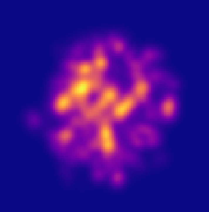
Following the “Working with Python” example in the TRENTO documentation, read the events in events.hdf and display the grids of several events with different impact parameters.
Describe the structure of the data: what is stored for each event, and what are the units of the grid coordinates? What quantity is on the “z” (colour) axis? Read Ref. [2], and the description of
multin the TRENTO documentation.Verify numerically that
multequals the sum of the grid values times the area of a grid cell, \((0.2\ \mathrm{fm})^2\).Plot the distributions of
b,npartandmultfor all events.
Question 05#
Centrality is defined by ranking events by the amount of particle production. The file contains minimum-bias events, so you have to select centrality classes yourself.
Sort the events by
mult(largest first), and assign each event a centrality percentile.Plot
bandnpartas functions of centrality.Select the events in the 5–10% centrality class, which we will compare with ATLAS data. How many events are there? What range of impact parameters do they span?
Question 06#
The eccentricities stored with each event follow Ref. [2]. Their magnitudes, together with an angle \(\Phi_n\) that we define here, are
where \(T_R\) is the grid value and \((r, \phi)\) are measured from the centre of mass of the event. Note the weight \(r^n\). The minus sign is our convention for the angle and does not affect \(\varepsilon_n\). Some other references, including the NuclearGeometryQGP projects, use \(r^2\) for all \(n\).
Write a function that computes \(\varepsilon_n\) and the angle \(\Phi_n\) from a grid. Check that it reproduces the stored
e2–e5.Draw the direction \(\Phi_2\) on top of a few event images. Because of the minus sign in the definition, \(\Phi_2\) points along the short axis of the overlap region. Why is this the direction in which we expect the most jets to survive?
Plot \(\langle\varepsilon_2\rangle\) and \(\langle\varepsilon_3\rangle\) as functions of centrality, and explain their behaviour.
Part D: Jets and energy loss#
Question 07#
Explore jet_energy.txt.
Plot the distribution of jet energies on a logarithmic scale.
Look at consecutive values in the file. Do you notice a pattern? Plot the distribution separately for the even-numbered and odd-numbered lines, and compare them value by value.
What do you conclude about how this jet sample was generated? In particular, look at the region below about 100 GeV.
Why does this matter if we want to model jets in ATLAS’s measured range, 71–398 GeV, after they have lost energy?
Fit a power law \(dN/dE \propto E^{-n}\) to the distribution where it is unbiased (e.g., by maximum likelihood). We will use it as the initial jet spectrum in the next questions.
Question 08#
Ref. [3] models the energy loss of a jet in the QGP (their Eqs. (1) and (2)) as a function of the jet energy \(E(\tau)\), the energy density of the medium \(e(\tau)\), and the path length \(\tau\) travelled by the jet. We use a slightly generalized form with four parameters:
The minus sign makes the jet lose energy for \(\kappa > 0\). The radiative (pQCD) case of Ref. [3], their Eq. (2), corresponds to \(\alpha = 0\), \(\beta = 3/4\), \(\gamma = 1\). As a simplification, we use the TRENTO grid \(T_R(x, y)\) as the medium density \(e\) and treat it as static. This neglects the expansion and cooling of the QGP.
Write a function that places a jet in a TRENTO event and lets it propagate through the medium, losing energy along the way:
Choose the starting point at random, with probability proportional to \(T_R^2\). Hard scatterings scale with the density of binary nucleon–nucleon collisions, \(\propto T_A T_B\). For TRENTO’s default parameter \(p = 0\), \(T_R = \sqrt{T_A T_B}\), so this is \(T_R^2\). The settings used to generate this file are not documented, so treat this as an approximation. Choose the direction uniformly in \([0, 2\pi)\).
Step the jet forward in small steps (\(d\tau = 0.2\) fm, one grid cell, works well). Interpolate the density at the jet position (e.g.,
scipy.ndimage.map_coordinates), and update \(E\). Stop when the jet leaves the grid or its energy reaches zero.Return the final energy and the jet direction relative to the event’s \(\Phi_2\).
Using one 5–10% event and the pQCD exponents, plot the fractional energy loss as a function of the jet direction relative to \(\Phi_2\), and as a function of the path length through the medium, for a few values of \(\kappa\). Explain what you see.
def eloss(event, E, kappa, alpha, beta, gamma, rng, dtau=0.2):
    """
    event : TRENTO grid (100 x 100 array)
    E     : array of initial jet energies (GeV)
    kappa, alpha, beta, gamma : energy-loss model parameters
    rng   : numpy random Generator (for reproducibility)
    Returns arrays of final jet energies and jet angles relative to the event's Phi_2.
    """
    ...
Question 09#
A first prediction. For the 5–10% centrality events, generate a large sample of jets. Draw the initial energies from your power-law spectrum from Question 07, propagate them with your Question 08 code (pQCD exponents, and a few values of \(\kappa\)), and compute the jet \(v_2\) in each of ATLAS’s \(p_T\) bins (defined in the cell below) using your vn function from Question 03. At the LHC, jets are so energetic that they are effectively massless, so \(p_T \approx E\) for our purposes.
Estimate the statistical uncertainty of each \(v_2\) value by subsampling: compute \(v_2\) for many independent sub-samples, and use the spread of the results. Compare it with the expectation from Question 03.
Plot your predictions together with the ATLAS data (Fig. 7 of Ref. [4]), and the inclusive 71–398 GeV value (Fig. 8 of Ref. [4]). How does \(v_2\) depend on \(\kappa\)? Is there a value that describes the data reasonably well?
Very few jets end up in the highest \(p_T\) bins. How could you reduce the statistical uncertainty there without simulating far more jets? (Hint: importance sampling.)
You will fit the model parameters properly in Project 02.
# ATLAS jet v2 for 5-10% centrality Pb+Pb collisions, Fig. 7 of Ref. [4], digitized with https://plotdigitizer.com/app.
# Exact values (with separate statistical and systematic uncertainties) are available on HEPData (record ins1967021).
pt_bin_edges = np.array([71, 79, 89, 100, 126, 158, 200, 251, 316, 398])   # GeV; 9 bins
v2_values = np.array([0.0248856, 0.0221773, 0.0195450, 0.0180492, 0.0178510,
                      0.0086814, 0.0120297, 0.0036979, 0.0138812])
v2_errors = np.array([0.0050671, 0.0049263, 0.0042100, 0.0038375, 0.0038205,
                      0.0041046, 0.0048910, 0.0053504, 0.0092933])
References#
[1] S. A. Voloshin, A. M. Poskanzer, R. Snellings, “Collective phenomena in non-central nuclear collisions,” in Relativistic Heavy Ion Physics, Landolt-Börnstein I/23, 293 (Springer, 2010). doi:10.1007/978-3-642-01539-7_10, arXiv:0809.2949
[2] J. S. Moreland, J. E. Bernhard, S. A. Bass, “Alternative ansatz to wounded nucleon and binary collision scaling in high-energy nuclear collisions,” Phys. Rev. C 92, 011901 (2015). doi:10.1103/PhysRevC.92.011901, arXiv:1412.4708. Code documentation: http://qcd.phy.duke.edu/trento/
[3] B. Betz, F. Senzel, C. Greiner, M. Gyulassy, “The impact of the medium and the jet-medium coupling on jet measurements at RHIC and LHC,” arXiv preprint (2015). arXiv:1512.07443
[4] ATLAS Collaboration, “Measurements of azimuthal anisotropies of jet production in Pb+Pb collisions at √sNN = 5.02 TeV with the ATLAS detector,” Phys. Rev. C 105, 064903 (2022). doi:10.1103/PhysRevC.105.064903, arXiv:2111.06606. Numerical data: HEPData
[5] W. Busza, K. Rajagopal, W. van der Schee, “Heavy Ion Collisions: The Big Picture, and the Big Questions,” Ann. Rev. Nucl. Part. Sci. 68, 339 (2018). doi:10.1146/annurev-nucl-101917-020852, arXiv:1802.04801
Acknowledgements#
Initial version: Abraham Holterman with some guidance from Mark Neubauer
Revised: 2026
© Copyright 2026