Aberrated Image Recovery of Ultracold Atoms

Aberrated Image Recovery of Ultracold Atoms#

%matplotlib inline
import matplotlib.pyplot as plt
import seaborn as sns; sns.set()
import numpy as np
import pandas as pd
import scipy as sp
import skimage as ski

Overview#

Over the past 20-30 years the groundwork has been lain for precise experimental control of atomic gases at ultracold temperatures. These ultracold atom gas experiments explore the quantum mechanics of their underlying atomic systems to a diverse set applications ranging from the simulation of computationally intractable physics problems [1] to the sensing of new physics beyond the standard model [2]. Most experiments in this field rely on directly imaging the ultracold gas they make, in order to extract data about the size and shape of the atomic number density distribution being imaged.

The goal of this project is introduce you to some image processing techniques from the world of data science and machine learning, as well as to get familiar with an image as a data element. As you will demonstrate, images are a kind of data with a very large number of features, but where almost all of those features within some region of interest are highly correlated. Of interest in this project is how the effects of real imaging systems distort the information contained in an image, and how those effects can be unfolded from the data to recover information about the true density distribution.

Capturing all possible kinds of aberrations and noise present in real experimental data of ultracold atom images is outside the scope of the simulated test data in this project. Instead, we limit ourselves to few a key effects: optical aberrations in the form of defocus and primary spherical aberrations, pixelization from a finite detector resolution, and at times toy number density noise simulated as simply Gaussian noise.

Data Sources#

Data is available here on the course GitHub, along with ImageSimulation.ipynb, the notebook used to generate the data. You are encouraged to read through that notebook to see how the simulation works and even generate your own datasets if desired.

You are welcome to access the images however works best for you, but a simple solution is to download the dataset folder to the same path where this notebook (or the one you plan to do your analysis in) is and use the following helper function to important an image based on the true parameters of the underlying density distribution—found in the image file name.

def Import_Image(dataset_name, imaging_sys, atom_number, mu_x, mu_y, mu_z, sigma_x, sigma_y, sigma_z, Z_04, seed):
    """Important an image following the project file naming structure.
    
    :param dataset_name: str
        Name of the dataset.
    :param imaging_sys: str
        Name of the imaging system (e.g. 'LoNA' or 'HiNA').
    :param atom_number: int
        Atom number normalization factor. 
    :param mu_x: float
        Density distribution true mean x.
    :param mu_y: float
        Density distribution true mean y.
    :param mu_z: float
        Density distribution true mean z.
    :param sigma_x: float
        Density distribution true sigma x.
    :param sigma_y: float
        Density distribution true sigma y.
    :param sigma_z: float
        Density distribution true sigma z.
    :param Z_04: float
        Coefficient of spherical aberrations.
    :param seed: int
        Seed for Gaussian noise.
    :return: 
    """
    dataset_name = dataset_name + '\\'
    file_name = imaging_sys + 'atom_num=%i.mu=(%0.1f...%0.1f...%0.1f).sigma=(%0.1f...%0.1f...%0.1f).Z04=%0.1f.seed=%i.tiff' % (atom_number, mu_x, mu_x, mu_z, sigma_x, sigma_y, sigma_z, Z04, seed)
    im = ski.io.imread(dataset_name + file_name)
    return im

Questions#

Question 01#

What is a cold atom gas? How cold are we talking? How do experiments bring atoms down to those temperatures?

When you research these experiments you will find that the Alkali atoms (Rb, K, Na, etc.) compose the majority set of species used. Why these atoms? Hint: recall high school chemistry. What do these atoms have in common with everyone’s favorite quantum system, the hydrogen atom?

A helpful resource is Foot’s Atomic Physics [3].

Question 02#

When attempting to measure the number density distribution of cold atom gas in experiment, we typically release the gas from any kind of confinement it was in and let it expand in free-fall before taking an image. When we take a picture thereafter the density distribution often has the shape of Gaussian. Why is that? Think stat mech.

Question 03#

Real imaging systems have a finite resolution set by the diffraction limit. Given a point source emitting a spherical EM field, a real lens will propagate the field from the object plane to the imaging plane, projecting a pattern which we call the imaging response function, or point spread function (PSF), of the system. For any object with finite size, we can think of the resultant image as being formed by a sum over the PSF associated with each point in the object, i.e. a convolution.

For a circular lens the shape of the best focus PSF (meaning the shape of an image formed from a point source located on the imaging axis at the best focus) we refer to as the Airy disk. Its first set of zeros are located at \(\rho\approx3.83\), for a dimensionless radial component \(\rho\).

Given this information and the functional form of the Airy disk, estimate the amount of irradiance (or weight) that sits in the central peak of the pattern relative to the whole distribution.

If you were to approximate this distribution to a Gaussian with the same peak irradiance, how would the first minima of the Airy disk relate to the \(1/e^2\) waist of the Gaussian distribution?

In addition to provided links, another useful resource is Goodman’s Introduction to Fourier Optics [4].

Questions 04#

In the previous question the resolution we were interested in describes the size of the image of a point source in the plane transverse to the axis the image propagates along. What about along the imaging axis? We often calls this axial resolution the depth of field (DOF), although when we want a number to describe it different sources define that value differently.

How are the DOF and transverse resolution related to each other? No mathematical relationship is necessary here (although you can if you want to, so long as you restrict yourself to thinking about the axial PSF along \(\rho=0\)).

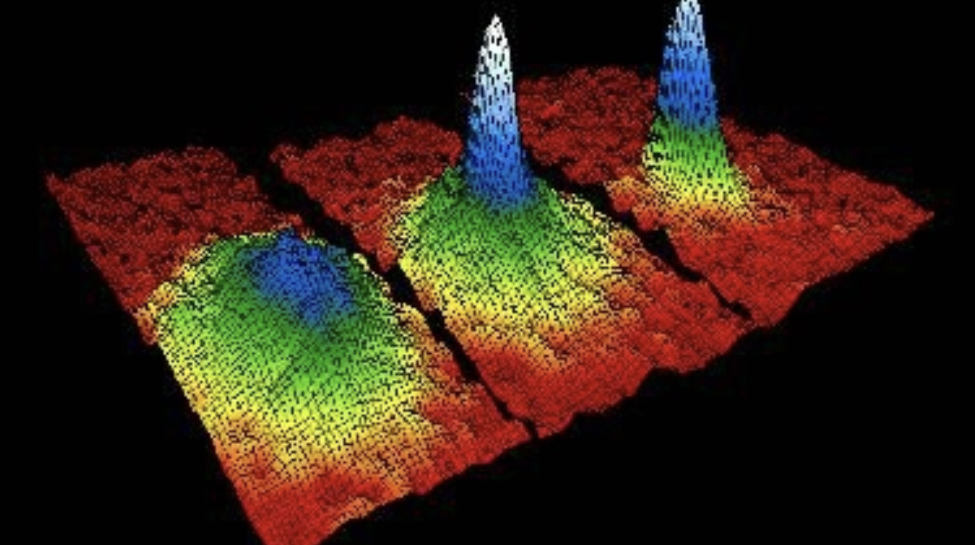
To answer the rest of the questions in first chunk of this project we will use images from the Number_estimate and Heavy_tails datasets. This data was generated in the ImageSimulation.ipynb, found at the link above. The images in the Heavy_tails dataset depict cold atom gases of variable \(\sigma_{xy}\) and \(\sigma_z\) at an arbitrary atom number, and those in the Number_estimate dataset contain images of a large isotropic (\(\sigma_{xy}=\sigma_z=20\) um) gas across a range of atom numbers and with number noise varying from shot to shot.

In generating these images, there are handful of fixed hyperparameters chosen to match a realistic set of experimental conditions. Here we are imaging a thermal gas of Rb\(^{87}\) atoms with a \(\lambda=780\) nm (near-infrared) light. That light is collected as by one of two imaging system: a (relatively) high numerical aperture (\(\text{NA}=0.4\)) lens and a lower resolution (\(\text{NA}=0.2\)) one. The image is projected on to a camera sensor with a pixel size of \(\text{PS}=13\) um, by a telescope with and \(\text{M}=20\times\) or \(\text{M}=4\times\) magnification respectively for each lens.

The images in the Heavy_tails dataset were generated with the high NA system and no number noise and the those in Number_estimate dataset were generated with the low NA system including number noise.

With the Number_estimate dataset you will explore how noise effects your ability to accurately estimate the total number of atoms in an image. Please ImageSimulation.ipynb for a fuller explanation as to what this noise represents.

With the Heavy_tails dataset you will test the ability of a simple linear decomposition to reduce the dimensionality of the data and confirm whether the ‘compressed’ image still retains relevant features of the gas. Images involving gases generated with \(\sigma_z\gtrsim \text{DOF}\) will acquire a noticeable tail in the image, diverging from the true Gaussian number density distribution. Of interest is how this tail is carried through to the compressed and reconstructed images.

Question 06#

The data here in this project are images—2D arrays containing greyscale information of the irradiance associated with the image of the gas. What is the dimension of this kind of data?

Consider the Number_estimate dataset of images and take each image as a sample across all dimensions of the image data. Suppose the question we are interested in is: Can we determine that the number of atoms in the image is greater than \(X\)? How many samples would we need to fully sample the parameter space of images here if none of the pixels in an image were correlated?

Quesiton 07#

Take images from the Number_estimate dataset where the total atom number of true distribution is \(N=100000\) and draw an appropriately binned histogram of the total atom number in the image by summing over all the pixels in the image. Repeat this for the \(N=10000\) subset of the dataset.

Note: in reality the total atom number in these kind of images doesn’t come directly from the

How are these histograms distinct from each other?

Question 08#

Draw histograms for the rest of the data in the Number_estimate dataset. Implement a KMeans fit of the 1D atom number data to attempt to recover the true atom number of each image, when comparing images in the following subsets of atom numbers: (7000, 10000, 13000), (70000, 100000, 130000), and (97000, 100000, 103000).

Are you able to clearly resolve the atom number for each of the subsets above?

Question 09#

Take the images in the Heavy_tails dataset. Use singular value decomposition (SVD) to generate a compressed version of each image, by decomposing the data and sampling a rank-\(k\) subset of the latent variable space. Reconstruct images for a handful of \(k\).

At what point do images with the same \(\sigma_{xy}\) but different \(\sigma_z\) appear to have the same sized tail in the compressed parameter space?

References#

[1] S. S. Kondov, W. R. McGehee, J. J. Zirbel, and B. DeMarco, Science 334, 66 (2011).
[2] W. B. Cairncross, D. N. Gresh, M. Grau, K. C. Cossel, T. S. Roussy, Y. Ni, Y. Zhou, J. Ye, and E. A. Cornell, Physical Review Letters 119, (2017).
[3] Goodman, J. W. (2005). Introduction to Fourier optics. 3rd ed.
[4] Foot, C. (2005). Atomic physics. Oxford University Press, USA.

Acknowledgements#

Initial version: Max Gold with some guidence from Mark Neubauer

Aberrated Image Recovery of Ultracold Atoms

Contents

Aberrated Image Recovery of Ultracold Atoms#

Overview#

Overview#

Data Sources#

Questions#

Question 01#

Question 02#

Question 03#

Questions 04#

Question 06#

Quesiton 07#

Question 08#

Question 09#

References#

Acknowledgements#