Statistics

%matplotlib inline
import matplotlib.pyplot as plt
import seaborn as sns; sns.set()
import numpy as np
import pandas as pd
import os
import subprocess

import scipy.stats

Data helpers

def wget_data(url):
    local_path='./tmp_data'
    subprocess.run(["wget", "-nc", "-P", local_path, url])

def locate_data(name, check_exists=True):
    local_path='./tmp_data'
    path = os.path.join(local_path, name)
    if check_exists and not os.path.exists(path):
        raise RuxntimeError('No such data file: {}'.format(path))
    return path

Get Data

wget_data('https://raw.githubusercontent.com/illinois-ipaml/MachineLearningForPhysics/main/data/blobs_data.hf5')

File ‘./tmp_data/blobs_data.hf5’ already there; not retrieving.

Load Data

blobs = pd.read_hdf(locate_data('blobs_data.hf5'))

Statistical Methods

The boundary between probability and statistics is somewhat gray (similar to astronomy and astrophysics). However, you can roughly think of statistics as the applied cousin of probability theory.

Expectation

Given a probability density \(P(x,y)\), and an arbitrary function \(g(x,y)\) of the same random variables, the expectation value of \(g\) is defined as:

\[ \Large \langle g\rangle \equiv \iint dx dy\, g(x,y) P(x,y) \; . \]

Note that the result is just a number, and not a function of either \(x\) or \(y\). Also, \(g\) might have dimensions, which do not need to match those of the probability density \(P\), so \(\langle g\rangle\) generally has dimensions.

Sometimes the assumed PDF is indicated with a subscript, \(\langle g\rangle_P\), which is helpful, but more often not shown.

When \(g(x,y) = x^n\), the resulting expectation value is called a moment of x. (The same definitions apply to \(y\), via \(g(x,y) = y^n\).) The case \(n=0\) is just the normalization integral \(\langle \mathbb{1}\rangle = 1\). Low-order moments have familiar names:

• \(n=1\) yields the mean of x, \(\overline{x} \equiv \langle x\rangle\).

• \(n=2\) yields the root-mean square (RMS) of x, \(\langle x^2\rangle\).

Another named expectation value is the variance of x, which combines the mean and RMS,

\[ \Large \sigma_x^2 \equiv \langle\left( x - \overline{x} \right)^2\rangle \; , \]

where \(\sigma_x\) is called the standard deviation of x.

Finally, the correlation between x and y is defined as: $\( \Large \text{Corr}_{xy} \equiv \langle\left( x - \overline{x}\right) \left( y - \overline{y}\right)\rangle \; . \)$

A useful combination of the correlation and variances is the correlation coefficient,

\[ \Large \rho_{xy} \equiv \frac{\text{Corr}_{x,y}}{\sigma_x \sigma_y} \; , \]

which, by construction, must be in the range \([-1, +1]\). Larger values of \(|\rho_{xy}|\) indicate that \(x\) and \(y\) are measuring related properties of the outcome so, together, carry less information than when \(\rho_{xy} \simeq 0\). In the limit of \(|\rho_{xy}| = 1\), \(y = y(x)\) is entirely determined by \(x\), so carries no new information.

We say that the variance and correlation are both second-order moments since they are expectation values of second-degree polynomials.

We call the random variables \(x\) and \(y\) uncorrelated when:

\[ \Large x,y\, \text{uncorrelated}\quad\Rightarrow\quad \text{Corr}_{xy} = \rho_{xy} = 0 \; . \]

To obtain an empirical estimate of the quantities above derived from your data, use the corresponding numpy functions, e.g.

np.mean(blobs, axis=0)

x0    6.920270
x1    4.502004
x2    8.492347
dtype: float64

np.var(blobs, axis=0)

x0    12.684951
x1     6.807913
x2    15.503924
dtype: float64

np.std(blobs, axis=0)

x0    3.561594
x1    2.609198
x2    3.937502
dtype: float64

assert np.allclose(np.std(blobs, axis=0) ** 2, np.var(blobs, axis=0))

assert np.allclose(
    np.mean((blobs - np.mean(blobs, axis=0)) ** 2, axis=0),
    np.var(blobs, axis=0))

The definition

\[ \Large \sigma_x^2 = \langle\left( x - \overline{x} \right)^2\rangle \]

suggests that two passes through the data are necessary to calculate variance: one to calculate \(\overline{x}\) and another to calculate the residual expectation. Expanding this definition, we obtain a formula

\[ \Large \sigma_x^2 = \langle x^2\rangle - \langle x\rangle^2 \]

that can be evaluated in a single pass by simultaneously accumulating the first and second moments of \(x\). However, this approach should generally not be used since it involves a cancellation between relatively large quantities that is subject to large round-off error. More details and recommended one-pass (aka “online”) formulas are here.

Covariance

It is useful to construct the covariance matrix \(C\) with elements:

\[\begin{split} \Large C \equiv \begin{bmatrix} \sigma_x^2 & \rho_{x,y} \sigma_x \sigma_y \\ \rho_{x,y} \sigma_x \sigma_y & \sigma_y^2 \\ \end{bmatrix} \end{split}\]

With more than 2 random variables, \(x_0, x_1, \ldots\), this matrix generalizes to:

\[ \Large C_{ij} = \langle \left( x_i - \overline{x}_i\right) \left( x_j - \overline{x}_j\right)\rangle \; . \]

Comparing with the definitions above, we find variances on the diagonal:

\[ \Large C_{ii} = \sigma_i^2 \]

and symmetric correlations on the off-diagonals:

\[ \Large C_{ij} = C_{ji} = \rho_{ij} \sigma_i \sigma_j \; . \]

(The covariance is not only symmetric but also positive definite).

The covariance matrix is similar to a pairplot, with each \(2\times 2\) submatrix

\[\begin{split} \Large \begin{bmatrix} \sigma_i^2 & \rho_{ij} \sigma_i \sigma_j \\ \rho_{ij} \sigma_i \sigma_j & \sigma_j^2 \\ \end{bmatrix} \end{split}\]

describing a 2D elllipse in the \((x_i, x_j)\) plane:

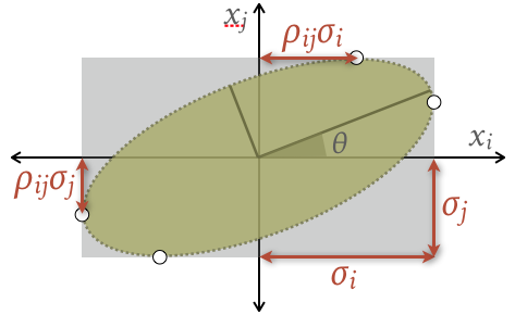
Note that you can directly read off the correlation coefficient \(\rho_{ij}\) from any of the points where the ellipse touches its bounding box. The ellipse rotation angle \(\theta\) is given by:

\[ \Large \tan 2\theta = \frac{2 C_{ij}}{C_{ii} - C_{jj}} = \frac{2\rho_{ij}\sigma_i\sigma_j}{\sigma_i^2 - \sigma_j^2} \]

and its principal axes have lengths:

\[ \Large a_\pm = 2\sqrt{C_{ii} + C_{jj} \pm d} \quad \text{with} \quad d = \sqrt{C_{11}^2 - 2 (1 - 2\rho^2) C_{11} C_{22} + C_{22}^2} \; . \]

For practical calculations, the Singular Value Decomposition (SVD) of the covariance is useful:

U, s, _ = np.linalg.svd(C)
theta = np.arctan2(U[1, 0], U[0, 0])
ap, am = 2 * np.sqrt(s)

The above assumes \(C\) is \(2\times 2\). In the general \(D\times D\) case, use C[[[j], [i]], [[j, i]]] to pick out the \((i,j)\) \(2\times 2\) submatrix.

A multivariate Gaussian PDF integrated over this ellipse (and marginalized over any additional dimensions) has a total probability of about 39%, also known as its confidence level (CL). We will see below how to calculate this CL and scale the ellipse for other CLs.

EXERCISE: Calculate the empirical covariance matrix of the blobs dataset using np.cov (pay attention to the rowvar arg). Next, calculate the ellipse rotation angles \(\theta\) in degrees for each of this matrix’s 2D projections.

C = np.cov(blobs, rowvar=False)
for i in range(3):
    for j in range(i + 1, 3):
        U, s, _ = np.linalg.svd(C[[[j], [i]], [[j, i]]])
        theta = np.arctan2(U[1, 0], U[0, 0])
        print(i, j, np.round(np.degrees(theta), 1))

0 1 123.3
0 2 -138.2
1 2 151.0

Recall that the blobs data was generated as a mixture of three Gaussian blobs, each with different parameters. However, describing a dataset with a single covariance matrix suggests a single Gaussian model. The lesson is that we can calculate an empirical covariance for any data, whether or not it is well described a single Gaussian.

Jensen’s Inequality

Convex functions play a special role in optimization algorithms (which we will talk more about soon) since they have a single global minimum with no secondary local minima. The parabola \(g(x) = a (x - x_0)^2 + b\) is a simple 1D example, having its minimum value of \(b\) at \(x = x_0\), but convex functions can have any dimensionality and need not be parabolic (second order).

Expectations involving a convex function \(g\) satisfy Jensen’s inequality, which we will use later:

\[ \Large g(\langle \vec{x} \ldots\rangle) \le \langle g(\vec{x})\rangle \; . \]

In other words, the expectation value of \(g\) is bounded below by \(g\) evaluated at the PDF mean, for any PDF. Note that the two sides of this equation swap the order in which the operators \(g(\cdot)\) and \(\langle\cdot\rangle\) are applied to \(\vec{x}\).

def jensen(a=1, b=1, c=1):
    x = np.linspace(-1.5 * c, 1.5 * c, 500)
    g = a * x ** 2 + b
    P = (np.abs(x) < c) * 0.5 / c
    plt.fill_between(x, P, label='$P(x)$')
    plt.plot(x, P)
    plt.plot(x, g, label='$g(x)$')
    plt.legend(loc='upper center', frameon=True)
    plt.axvline(0, c='k', ls=':')
    plt.axhline(b, c='r', ls=':')
    plt.axhline(a * c ** 2 + b, c='b', ls=':')
    plt.xlabel('$x$')
    
jensen()

EXERCISE: Match the following values to the dotted lines in the graph above of the function \(g(x)\) and probability density \(P(x)\):

1. \(\langle x\rangle = \int dx\, x P(x)\)

2. \(\langle g(x)\rangle = \int dx\, g(x)\,P(x)\)

3. \(g(\langle x\rangle) = g\left( \int dx\, x P(x)\right)\)

Is \(g(x)\) convex? Is Jensen’s inequality satisfied?

Answer:

1. Vertical (black) line.

2. Upper horizontal (blue) line.

3. Lower horizontal (red) line.

Jensen’s inequality is satisfied, as required since \(g(x)\) is convex.

Acknowledgments

• Initial version: Mark Neubauer

© Copyright 2024