Aberrated Image Recovery of Ultracold Atoms#
%matplotlib inline
import matplotlib.pyplot as plt
import seaborn as sns; sns.set_theme()
import numpy as np
import pandas as pd
import scipy as sp
import skimage as ski
import sklearn as skl
from sklearn import cluster
Overview#
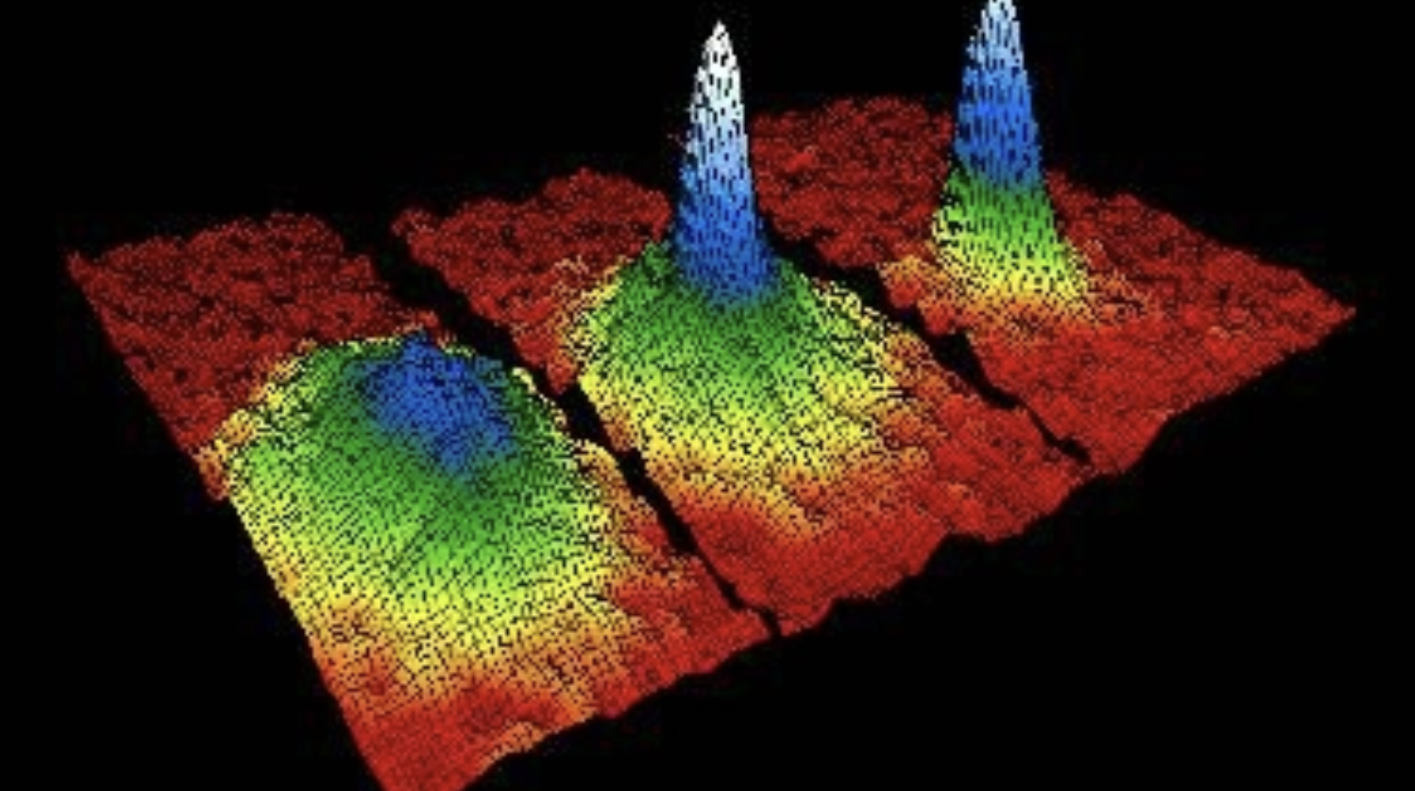
Over the past 20-30 years the groundwork has been laid for precise experimental control of atomic gases at ultracold temperatures. These ultracold atom gas experiments explore the quantum mechanics of their underlying atomic systems to a diverse set applications ranging from the simulation of computationally difficult physics problems [1] to the sensing of new physics beyond the standard model [2]. Most experiments in this field rely on directly imaging the ultracold gas they make, in order to extract data about the size and shape of the atomic number density distribution being imaged.
The goal of this project is to introduce you to some relevant image processing techniques, as well as to get familiar with an image as a data element. As you will demonstrate, images are a kind of data with a very large number of features, but where almost all of those features within some region of interest are highly correlated. Of interest in this project is how the effects of real imaging systems distort the information contained in an image, and how those effects can be unfolded from the data to recover information about the true density distribution.
Capturing all possible kinds of aberrations and noise present in real experimental data of ultracold atom images is outside the scope of the simulated test data in this project. Instead, we limit ourselves to a few key effects: optical aberrations in the form of defocus and primary spherical aberrations, pixelization from a finite detector resolution, and at times toy number density noise simulated as simple Gaussian noise.
Data Sources#
File URLs
You should untar this file into your local directory and access the image files from there:
Heavy_tails/HiNA.atom_num=100000.*.tiff
Also included is ImageSimulation.ipynb, which is the notebook used to generate the data you will find in that folder. You are encouraged to read through that notebook to see how the simulation works and even generate your own datasets if desired.
You are welcome to access the images however works best for you, but a simple solution is to download the dataset folder to the same path as this notebook (or the one you plan to do your analysis in) and use the following helper function to important an image based on the true parameters of the underlying density distribution—found in the image file name.
def Import_Image(dataset_name, imaging_sys, atom_number, mu_x, mu_y, mu_z, sigma_x, sigma_y, sigma_z, Z04, seed):
    """Important an image following the project file naming structure.

    :param dataset_name: str
        Name of the dataset.
    :param imaging_sys: str
        Name of the imaging system (e.g. 'LoNA' or 'HiNA').
    :param atom_number: int
        Atom number normalization factor.
    :param mu_x: float
        Density distribution true mean x.
    :param mu_y: float
        Density distribution true mean y.
    :param mu_z: float
        Density distribution true mean z.
    :param sigma_x: float
        Density distribution true sigma x.
    :param sigma_y: float
        Density distribution true sigma y.
    :param sigma_z: float
        Density distribution true sigma z.
    :param Z04: float
        Coefficient of spherical aberrations.
    :param seed: int
        Seed for Gaussian noise.
    :return:
    """
    dataset_name = dataset_name + '\\'
    file_name = imaging_sys + '.atom_num=%i.mu=(%0.1f...%0.1f...%0.1f).sigma=(%0.1f...%0.1f...%0.1f).Z04=%0.1f.seed=%i.tiff' % (atom_number, mu_x, mu_y, mu_z, sigma_x, sigma_y, sigma_z, Z04, seed)
    im = ski.io.imread(dataset_name + file_name)
    return im
Questions#
Please refer to the corresponding Project 01 notebook for background questions related to this project. In this project, you are to focus on machine learning application(s).
Question 01#
Take the images in the Heavy_tails dataset. Use singular value decomposition (SVD) to generate a compressed version of each image, by decomposing the data and sampling a rank-\(k\) subset of the latent variable space. Reconstruct images for a handful of \(k\).
At what point do images with the same \(\sigma_{xy}\) but different \(\sigma_z\) appear to have the same sized tail in the compressed parameter space?
Question 02#
Read through chapter 5 of [5], and implement a similarly structured convolutional neural network (CNN) to extract features from the images in the Heavy_tails dataset.
Display a few images from the output of the network? How do they compare to your latent space representations of the data from your SVD?
References#
[1] S. S. Kondov, W. R. McGehee, J. J. Zirbel, and B. DeMarco, Science 334, 66 (2011).
[2] W. B. Cairncross, D. N. Gresh, M. Grau, K. C. Cossel, T. S. Roussy, Y. Ni, Y. Zhou, J. Ye, and E. A. Cornell, Physical Review Letters 119, (2017).
[3] C. J. Schuler, Machine learning approaches to image deconvolution. Eberhard Karls University of Tübingen (2014).
[4] Herbel, J., Kacprzak, T., Amara, A., Refregier, A., & Lucchi, A. (2018). Fast point spread function modeling with deep learning. Journal of Cosmology and Astroparticle Physics, 2018(07), 054.
[5] R. J. Steriti and M. A. Fiddy, “Blind deconvolution of images by use of neural networks,” Opt. Lett. 19, 575-577 (1994)
Acknowledgements#
Initial version: Max Gold with some guidence from Mark Neubauer
© Copyright 2025