Fluid Dynamics of a Bent Pipe

Fluid Dynamics of a Bent Pipe#

Overview#

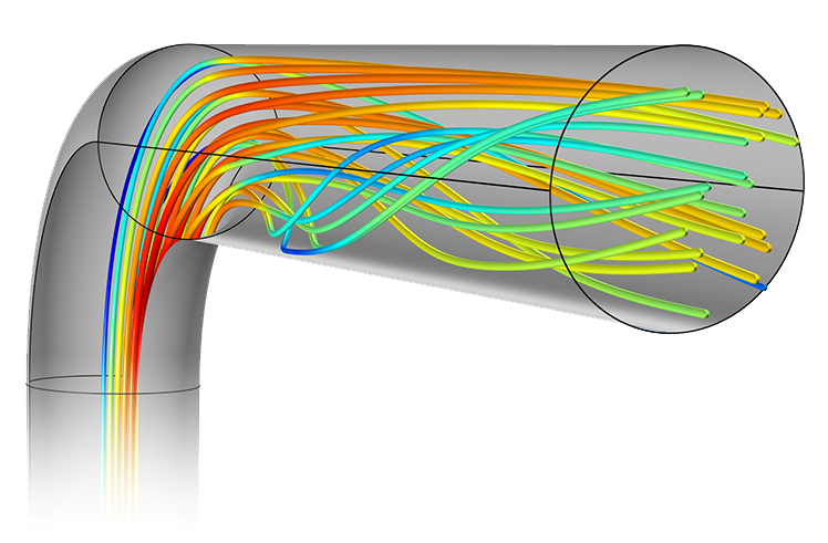
Computational fluid dynamics (CFD) simulations are essential but computationally expensive. A surrogate model trained on simulation results can predict the flow almost instantly, which makes real-time monitoring possible. In this project you will build surrogate models for the coolant flow in the “hot leg” of a pressurized-water nuclear reactor (a pipe with a 120° elbow), using CFD data from Ref. [1].

You will compare:

simple baselines that interpolate between stored simulations;
a fully connected feedforward neural network (FCFNN), which treats each point of the mesh independently; and
a graph neural network (GNN), which treats the mesh as a graph and passes messages between neighbouring points.

You will evaluate them on held-out simulations by their accuracy, their runtime, and their dependence on the Reynolds number. By the end of this project you should have a clear picture of when a neural-network surrogate is useful and when a simpler method wins.

Learning Objectives#

Explain why CFD simulations are expensive and what a surrogate model offers.
Prepare simulation output on an unstructured mesh for machine learning: masking, splitting by simulation, and normalization.
Implement a fully connected network and a message-passing graph neural network in PyTorch.
Evaluate surrogates fairly: with held-out simulations, appropriate error metrics, and simple baselines.

Questions 01 & 02: Motivation for creating a surrogate model#

Question 01: CFD runtime#

Why do traditional CFD simulations take so long to run? Visit Jose Alvarez and Mahmud Nobe’s notebook to learn more about the mathematics behind a CFD simulation (hint: the infamous Navier–Stokes equations). Ref. [1] reports how long its simulations took; how does that compare with the time needed to evaluate a trained neural network?

Data structure from the CFD simulation#

The data come from the CFD study of Ref. [1]. That study modelled a scaled-down (25 mm diameter) version of the hot leg of an AP1000 pressurized-water reactor, with a 120° elbow, an inlet temperature of 594.3 K, and turbulent flow. The paper ran 5000 simulations; this project uses a subset of 201 of them, available in the GitHub repository lightiet/bended_pipe (about 340 MB).

There are 201 files, axial_output_0.txt … axial_output_200.txt, one per simulation. Each simulation has a different inlet velocity \(U\), between about 0.66 and 0.80 m/s.
Each file lists 11,340 mesh nodes on the central plane of the pipe, with columns [nodenumber, x-coordinate, y-coordinate, z-coordinate, turb-kinetic-energy, pressure, temperature, velocity-magnitude], in SI units (m, m²/s², Pa (gauge), K, m/s).
The mesh is the same in every simulation. Because all nodes lie on one plane, the y-coordinate is constant.
324 nodes lie on the pipe wall, where the velocity is zero (the no-slip condition). We drop them.
The temperature is the same everywhere (594.3 K), so we ignore it.

# Download the data (about 340 MB); skip if already present
import os
if not os.path.isdir("bended_pipe"):
    !git clone --depth 1 https://github.com/lightiet/bended_pipe.git

Question 02: the 3 quantities#

Why is it important to monitor these three quantities in a reactor’s primary coolant loop? Ref. [1] discusses this in the context of materials degradation.

turbulent kinetic energy (TKE)
pressure
velocity

Data preparation#

import time
import numpy as np
import matplotlib.pyplot as plt
import torch
import torch.nn as nn
from torch.utils.data import Dataset, DataLoader
from sklearn.neighbors import NearestNeighbors

torch.manual_seed(42)
np.random.seed(42)
rng = np.random.default_rng(seed=42)
device = torch.device("cuda" if torch.cuda.is_available() else "cpu")
print("device:", device)

Question 03: Data preprocessing#

Prepare the data for training. Think about the goal of this project: what should the shape of the input and output vectors be?

Fill a NumPy array data_tensor of shape (num_sims, nodes_per_sim, 6) with the features [x, y, z, TKE, pressure, velocity].
Build a boolean mask over the nodes that keeps only the non-wall nodes (velocity ≠ 0), and apply it. Check that the wall nodes are the same in every simulation.

After masking, node index 2 lies on the inlet plane (\(z = 0\)), where the velocity is uniform. Its velocity is therefore the inlet velocity \(U\) of the simulation (see get_inlet_vel below). Verify this for a few simulations.

data_dir      = "bended_pipe/test_output_data"
file_pattern  = "axial_output_{}.txt"
num_sims      = 201
nodes_per_sim = 11340

# 1) Fill in the correct shape: (num_sims, nodes_per_sim, number_of_features)
#    Features: x, y, z, TKE, pressure, velocity
data_tensor = np.empty(...)  # YOUR CODE HERE

for i in range(num_sims):
    raw = np.loadtxt(os.path.join(data_dir, file_pattern.format(i)), skiprows=1)  # shape (11340, 8)
    raw = raw[raw[:, 0].argsort()]                                                 # sort by node number
    # 2) Select the columns [x, y, z, TKE, pressure, velocity]
    #    raw has columns [node#, x, y, z, TKE, pressure, temperature, velocity]
    data_tensor[i] = ...  # YOUR CODE HERE

# 3) Boolean mask over nodes, True where the velocity (last feature) is non-zero
mask = ...  # YOUR CODE HERE
data_tensor = data_tensor[:, mask, :]
print("data_tensor shape:", data_tensor.shape)

def get_inlet_vel(sim_idx):
    """Inlet velocity U of a simulation: node 2 (after masking) lies on the inlet plane, where the velocity is uniform."""
    return data_tensor[sim_idx, 2, 5]

U_all = np.array([get_inlet_vel(i) for i in range(num_sims)])
print(f"inlet velocities: {U_all.min():.3f} - {U_all.max():.3f} m/s")

# Split by *simulation* (not by node) into training and evaluation sets
perm      = rng.permutation(num_sims)
split_pt  = int(0.2 * num_sims)
eval_idx  = perm[:split_pt]
train_idx = perm[split_pt:]
train_tensor = data_tensor[train_idx]
eval_tensor  = data_tensor[eval_idx]
print("training tensor:", train_tensor.shape, " evaluation tensor:", eval_tensor.shape)

Reynolds number (Re)#

The Reynolds number is

\[ \Large Re = \frac{\rho U D}{\mu} \]

where \(\rho\) is the density of the coolant, \(U\) is the inlet velocity, \(D = 0.025\) m is the pipe diameter, and \(\mu\) is the dynamic viscosity.

It characterizes the flow regime. At low Re the flow is laminar and predictable, while at high Re it is turbulent and chaotic. For water at the reactor’s conditions (594.3 K and a typical primary-loop pressure of 15.5 MPa), \(\rho \approx 677\) kg/m³ and \(\mu \approx 8.0\times10^{-5}\) Pa·s. These values come from the IAPWS formulation, e.g. via the CoolProp package. Ref. [1] treats the coolant as having constant density and viscosity but does not quote the values it used, so treat these as representative.

RHO = 677.0     # kg/m^3, water at 594.3 K and 15.5 MPa
MU  = 8.0e-5    # Pa s
D   = 0.025     # m

def reynolds(U):
    return RHO * U * D / MU

print(f"Re range of the dataset: {reynolds(U_all.min()):.3g} - {reynolds(U_all.max()):.3g}")

Question 04: Predictability and Re#

Is the flow in this dataset laminar or turbulent? Based on what you just read, what do you expect the relationship between a surrogate model’s accuracy and Re to be? Note how wide (or narrow) the range of Re in this dataset is.

Visualizing the data#

The following code plots the three fields for the simulations with the lowest, median and highest inlet velocity, to help you gain intuition about the data.

order = np.argsort(U_all)
sim_indices = [order[0], order[len(order) // 2], order[-1]]
case_labels = ['lowest U', 'median U', 'highest U']
var_names   = ['TKE', 'Pressure', 'Velocity']
x, z = data_tensor[0, :, 0], data_tensor[0, :, 2]

for sim, label in zip(sim_indices, case_labels):
    fig, axs = plt.subplots(1, 3, figsize=(18, 5))
    for idx, name in enumerate(var_names):
        sc = axs[idx].scatter(x, z, c=data_tensor[sim, :, 3 + idx], s=5)
        fig.colorbar(sc, ax=axs[idx], label=name)
        axs[idx].set_title(name); axs[idx].set_xlabel("x (m)"); axs[idx].set_ylabel("z (m)"); axs[idx].set_aspect("equal")
    fig.suptitle(f"{label}: U = {U_all[sim]:.3f} m/s, Re = {reynolds(U_all[sim]):.3g}", fontsize=16)
    plt.tight_layout(rect=[0, 0.03, 1, 0.95]); plt.show()

How good does a surrogate need to be? Baselines first#

Before training neural networks, establish what simple methods achieve. We measure the error of a predicted field \(\hat f\) against the true field \(f\) of one simulation, separately for each quantity, as a relative \(L_2\) error normalized by the spatial variation of the true field:

\[ \epsilon = \frac{\lVert \hat f - f \rVert_2}{\lVert f - \bar f \rVert_2}, \]

where the norms run over all nodes and \(\bar f\) is the spatial mean. A pointwise relative error \(|\hat f - f|/|f|\) is misleading here, because pressure and TKE can be close to zero.

def rel_l2(pred, true):
    """Relative L2 error per field. pred, true: arrays of shape (N_nodes, 3) for [TKE, pressure, velocity]."""
    return np.linalg.norm(pred - true, axis=0) / np.linalg.norm(true - true.mean(axis=0), axis=0)

Question 05: Baselines#

Implement two baselines that use only the stored training simulations, and evaluate them on every simulation in the evaluation set:

Nearest neighbour: predict the fields of the training simulation whose inlet velocity is closest to \(U\).
Linear interpolation: interpolate each node’s values linearly in \(U\) between the two training simulations whose inlet velocities bracket \(U\).

Report the median rel_l2 for each field. Also perform a principal component analysis (SVD) of the training fields of each quantity, across simulations, after subtracting the mean field. What fraction of the variance between simulations is captured by the first mode? What does that tell you about how complicated the mapping from \(U\) to the flow field is?

# YOUR CODE HERE

Neural-network surrogates#

Now that we have established that CFD requires significant computational resources, we can see why it is not suitable for real-time prediction of a system’s state. Machine learning offers an alternative: a model trained on simulations of the system’s geometry can predict its state almost instantly. Two approaches follow; implement both and compare them with each other and with the baselines.

Because the y-coordinate is constant, we use \((x, z)\) as the spatial coordinates. Each node’s input features are therefore \([x, z, U]\), and its targets are \([\text{TKE}, \text{pressure}, \text{velocity}]\). The normalization statistics are computed from the training set only.

def node_inputs(tensor):
    """Per-node inputs [x, z, U] for every simulation in `tensor`: shape (n_sims, N_nodes, 3)."""
    n_sims, n_nodes, _ = tensor.shape
    xz = tensor[:, :, [0, 2]]
    U = np.repeat(tensor[:, 2, 5][:, None, None], n_nodes, axis=1)
    return np.concatenate([xz, U], axis=2)

X_train, Y_train = node_inputs(train_tensor), train_tensor[:, :, 3:6]
X_eval,  Y_eval  = node_inputs(eval_tensor),  eval_tensor[:, :, 3:6]

mu_in,  s_in  = X_train.reshape(-1, 3).mean(0), X_train.reshape(-1, 3).std(0)
mu_out, s_out = Y_train.reshape(-1, 3).mean(0), Y_train.reshape(-1, 3).std(0)
norm_stats = {"mu_in": mu_in, "s_in": s_in, "mu_out": mu_out, "s_out": s_out}

Question 06: Fully connected feedforward neural network (FCFNN)#

Start with the simplest method: an FCFNN that maps a single node’s inputs \([x, z, U]\) to its outputs \([\text{TKE}, \text{pressure}, \text{velocity}]\). Every node of every training simulation is one training example (about 1.8 million examples), so train with mini-batches.

Train it, plot the training loss, and save the model together with the normalization statistics, as in the cell below.

class FCFNN(nn.Module):
    def __init__(self, input_dim=3, hidden_dims=(128, 128, 128), output_dim=3):
        super().__init__()
        # YOUR CODE HERE

    def forward(self, x):
        # YOUR CODE HERE
        pass

fcfnn = FCFNN().to(device)
# YOUR CODE HERE: training loop on the normalized inputs/targets

torch.save({"model_state_dict": fcfnn.state_dict(), "norm_stats": norm_stats}, "fcfnn_checkpoint.pt")

Question 07: Graph neural network (GNN)#

Treat each mesh node as a node of a graph, whose behaviour is influenced by its neighbours, and capture these local interactions with a graph neural network [4], [5]. Construct a GNN that:

builds a \(k\)-nearest-neighbour graph from the \((x, z)\) coordinates (the mesh is the same for all simulations, so the graph is built once);
maps the normalized node features \([x, z, U]\) to a hidden representation with an encoder;
applies several message-passing layers: each node updates its representation using its own state and the mean of its neighbours’ states;
maps back to \([\text{TKE}, \text{pressure}, \text{velocity}]\) with a decoder.

Each training example is a whole simulation (one graph). Implement the missing pieces in plain PyTorch. You can implement the neighbour aggregation with torch.Tensor.index_add_.

hidden_dim    = 128
num_layers    = 3
learning_rate = 1e-3
epochs        = 15
k_neighbors   = 6

def build_knn_graph(coords, k):
    """
    coords: array (N, 2) of node coordinates.
    Returns edge_index, a LongTensor of shape (2, N*k): edge_index[0] = source node i,
    edge_index[1] = one of the k nearest neighbours of i (excluding i itself).
    """
    # YOUR CODE HERE (hint: sklearn.neighbors.NearestNeighbors)


class FlowDataset(Dataset):
    """One item = one simulation: normalized node inputs x (N, 3) and targets y (N, 3)."""
    def __init__(self, tensor, norm_stats):
        self.X = (node_inputs(tensor) - norm_stats["mu_in"]) / norm_stats["s_in"]
        self.Y = (tensor[:, :, 3:6] - norm_stats["mu_out"]) / norm_stats["s_out"]

    def __len__(self):
        return len(self.X)

    def __getitem__(self, idx):
        return (torch.tensor(self.X[idx], dtype=torch.float32),
                torch.tensor(self.Y[idx], dtype=torch.float32))


class GraphConvLayer(nn.Module):
    def __init__(self, dim):
        super().__init__()
        # linear maps for the node's own state and for the aggregated neighbour states
        # YOUR CODE HERE

    def forward(self, h, edge_index):
        # message passing: mean over neighbours, combine with own state, non-linearity (+ residual connection)
        # YOUR CODE HERE
        pass


class FlowGNN(nn.Module):
    def __init__(self, in_dim=3, hidden_dim=128, out_dim=3, n_layers=3):
        super().__init__()
        # encoder, n_layers GraphConvLayers, decoder
        # YOUR CODE HERE

    def forward(self, x, edge_index):
        # YOUR CODE HERE
        pass

Now train the GNN. The graph is the same for every simulation, so it is built once and moved to the device.

edge_index = build_knn_graph(data_tensor[0][:, [0, 2]], k_neighbors).to(device)
train_loader = DataLoader(FlowDataset(train_tensor, norm_stats), batch_size=1, shuffle=True)

gnn = FlowGNN(in_dim=3, hidden_dim=hidden_dim, out_dim=3, n_layers=num_layers).to(device)
optimizer = torch.optim.Adam(gnn.parameters(), lr=learning_rate)
criterion = nn.MSELoss()
for epoch in range(1, epochs + 1):
    # YOUR CODE HERE: loop over train_loader (x, y have a leading batch dimension of 1), plot/print the loss
    pass

torch.save({"model_state_dict": gnn.state_dict(), "norm_stats": norm_stats}, "gnn_checkpoint.pt")

Question 08: Predicting a whole flow field#

The function below loads a saved model and predicts the fields over the whole pipe for a given inlet velocity \(U\). Read it and make sure you understand each step.

coords_xz = data_tensor[0][:, [0, 2]]

def predict_fields(U, model_type):
    """Predict [TKE, pressure, velocity] at every node for inlet velocity U. Returns an array (N_nodes, 3)."""
    if model_type.upper() == "GNN":
        ckpt = torch.load("gnn_checkpoint.pt", map_location=device, weights_only=False)
        model = FlowGNN(in_dim=3, hidden_dim=hidden_dim, out_dim=3, n_layers=num_layers)
    elif model_type.upper() == "FCFNN":
        ckpt = torch.load("fcfnn_checkpoint.pt", map_location=device, weights_only=False)
        model = FCFNN()   # change the arguments here if you changed the architecture
    else:
        raise ValueError(f"Unsupported model_type: {model_type}")
    model.load_state_dict(ckpt["model_state_dict"])
    model.to(device).eval()
    ns = ckpt["norm_stats"]

    X = np.hstack([coords_xz, np.full((len(coords_xz), 1), U)])
    x_t = torch.tensor((X - ns["mu_in"]) / ns["s_in"], dtype=torch.float32, device=device)
    with torch.no_grad():
        out = model(x_t, edge_index) if model_type.upper() == "GNN" else model(x_t)
    return out.cpu().numpy() * ns["s_out"] + ns["mu_out"]

Question 09: Evaluating the models#

Runtime: time a single call of predict_fields for each model (exclude the first call, which includes loading and warm-up), and compare it with the time for a CFD simulation (Question 01).
Accuracy: for every simulation in the evaluation set, predict the fields at its own inlet velocity, and compute rel_l2 for each model. Compare the median errors with the baselines of Question 05.
Error maps: for one evaluation simulation, plot the predicted fields of both models next to the true fields, and plot maps of the absolute error divided by the range of each true field.

Which method works best for this use case, and why? Think about how many independent parameters describe this family of flows (Question 05), and what a network that maps coordinates to field values has to learn [6].

# YOUR CODE HERE

Question 10: Relationship between Re and error#

Plot the error of each model (and of the baselines) against Re for the simulations in the evaluation set. Was your expectation from Question 04 correct? Which matters more here: the physics of turbulence, or where a simulation lies within the range of the training data?

# YOUR CODE HERE

Question 11: Possible improvements (optional)#

What enhancements or modifications would you suggest for these surrogate models? Some ideas to test:

train longer, tune the learning rate, or use a learning-rate schedule;
encode the coordinates with Fourier features [6], so that the network can represent fine spatial structure;
predict the coefficients of the leading principal components from Question 05 as a function of \(U\), instead of predicting every node separately;
a DeepONet [2], the architecture used in Ref. [1];
test extrapolation: train only on simulations with \(U\) in the lower 80% of the range, and evaluate on the highest 20%. How do the networks and the interpolation baselines compare now?

In what kind of problem would a neural-network surrogate clearly beat interpolation between stored simulations? Think about problems with many input parameters, e.g. several boundary conditions or a varying geometry.

References#

[1] R. Hossain, F. Ahmed, K. Kobayashi, S. Koric, D. Abueidda, S. B. Alam, “Virtual sensing-enabled digital twin framework for real-time monitoring of nuclear systems leveraging deep neural operators,” npj Mater. Degrad. 9, 21 (2025). doi:10.1038/s41529-025-00557-y

[2] L. Lu, P. Jin, G. Pang, Z. Zhang, G. E. Karniadakis, “Learning nonlinear operators via DeepONet based on the universal approximation theorem of operators,” Nat. Mach. Intell. 3, 218 (2021). doi:10.1038/s42256-021-00302-5, arXiv:1910.03193

[3] J. Alvarez, M. Nobe, “The Ultimate Guide to Write Your First CFD Solver,” Jupyter notebook. https://colab.research.google.com/github/josealvarez97/The-Ultimate-Guide-to-Write-Your-First-CFD-Solver/blob/main/The_Ultimate_Guide_to_Write_Your_First_CFD_Solver.ipynb

[4] J. Gilmer, S. S. Schoenholz, P. F. Riley, O. Vinyals, G. E. Dahl, “Neural Message Passing for Quantum Chemistry,” Proc. ICML (2017). arXiv:1704.01212

[5] T. Pfaff, M. Fortunato, A. Sanchez-Gonzalez, P. W. Battaglia, “Learning Mesh-Based Simulation with Graph Networks,” Proc. ICLR (2021). arXiv:2010.03409

[6] M. Tancik et al., “Fourier Features Let Networks Learn High Frequency Functions in Low Dimensional Domains,” Proc. NeurIPS (2020). arXiv:2006.10739

Acknowledgements#

Initial version: Abdulaziz Alshohail with some guidance from Mark Neubauer
Revised: 2026